Demodulation and Envelope Analysis

In this article, which is the fifth in a series, This is the topic of Demodulation and Surrounding Analysis, which plays a fundamental role in diagnosis by vibration analysis in machines.

Articles on this topic already published were:

1 Introduction to vibration and envelope modulation

2 History of modulation in vibration analysis

3 Concept of modulation and its physical origin

4) Mathematical Foundations of Vibration Modulation

5 Demodulation and envelope analysis

5.1 Introduction

Modulation constitutes the mechanism through which mechanical defects transfer information to a higher frequency vibration. However, This information is “hidden” on the amplitude, frequency or phase of the carrier vibration, not being immediately visible in the original waveform nor, oftentimes, not conventional FFT spectrum.

A demodulation is the set of techniques designed to separate this information from the carrier, allowing to directly recover the signal associated with the mechanical phenomenon that originated the modulation.

In vibration analysis, This operation is commonly called surround analysis , and the signal recovered in this way is called immersive. It is currently one of the most effective techniques for early detection of defects in bearings., gears and other components subject to periodic impacts.

Figure 5.1 – General concept of analysis by envelope.

5.2 Why Conventional FFT Isn't Always Enough

A conventional FFT represents the distribution of energy across the different frequencies present in the signal.

When a defect is sufficiently developed — which already corresponds to a late stage of the four classic stages of bearing degradation — the energy produced by impacts can be observed directly in the spectrum.

Yet, during the initial stages of degradation, the situation is different.

The impacts present:

very low energy;
short duration;
broadband spectral content, consequence of its short duration.

Much of this energy excites structural resonances between a few kilohertz and tens of kilohertz.

As a consequence, the spectrum shows only a slight increase in energy in a high frequency band, without clearly revealing the frequency of repetition of impacts.

It is precisely this limitation that justifies the use of envelope analysis.

Figure 5.2 – Comparison between conventional FFT and envelope FFT for a bearing with incipient defect.

5.3 Surrounding concept

Consider again a damped response produced by an impact.

The observed vibration has two distinct components:

a rapid oscillation corresponding to the resonant frequency of the structure;
a slow variation in amplitude determined by the repetition of impacts.

The envelope corresponds precisely to this slow variation in amplitude.

Mathematically, the envelope corresponds to the module of the analytical signal, obtained from the measured signal x(t) through the Hilbert Transform H[·]:

z(t) = x(t) + j·H[x(t)]

(5.1)

the envelope being given by

A(t) = |z(t)|

(5.2)

This definition only has physical meaning if the signal is narrow band in relation to the carrier frequency (Bedrosian condition). It is precisely this requirement that forces the signal to be filtered around a resonance before calculating the envelope.: applied to the complete signal, without prior filtering, the Hilbert Transform produces an envelope dominated by the machine's low-frequency components and without useful physical interpretation.

From a physical point of view, the envelope only describes the intensity of the vibration over time, eliminating the rapid oscillation associated with the carrier.

Figure 5.3 – Relationship between the original vibration, the envelope and the corresponding spectrum.

5.4 Surround analysis steps

Regardless of the algorithm used by the analyzer, processing can be divided into seven fundamental steps.

Acquisition

The accelerometer measures the total vibration of the machine, with a sampling frequency sufficient to cover the range of resonances excited by impacts.

Bandpass filtering

A frequency band is selected where there is a structural resonance excited by impacts. This filtering eliminates low-frequency components associated with imbalance, misalignment and gearing, that would otherwise dominate the outcome, and ensures the narrowband condition required by demodulation.

Demodulation

The high-frequency vibration is converted into its surroundings, usually through the Hilbert Transform.

Resampling (decimation)

The envelope has a much lower bandwidth than the original signal, so it can be determined without loss of information. It should be noted that the frequency resolution of the final spectrum continues to be determined exclusively by the duration of the recording, Δf = 1/T, that decimation does not change. What decimation allows is to concentrate the available spectral lines in the narrow band where the diagnostic information resides., typically a few kilohertz, instead of distributing them across the entire purchasing range, which can extend to tens of kilohertz. For the same number of lines we obtain, like this, a much smaller line spacing in the band of interest, simultaneously reducing the volume of data to be processed. This operation, often omitted in the method description, This is what makes it feasible to obtain the necessary resolution in the envelope spectrum to separate sidebands spaced at 1×RPM..

Removal of the continuous component

The surroundings are always a positive sign, with high average value. Without subtracting this continuous component, the spectrum is dominated by a line 0 Hz that compresses the scale and hides diagnostic streaks.

FFT of the envelope

Calculate the Fourier Transform of the envelope, typically with a Hanning window and an appropriate number of averages.

Diagnosis

The characteristic frequencies of the defect, their harmonics and respective sidebands become clearly visible.

This sequence currently constitutes the reference method for bearing diagnosis..

Figure 5.4 – Complete stages of analysis by envelope in a modern analyzer.

5.5 Demodulation methods

Throughout the evolution of instrumentation, several methods were developed to extract the surrounding. The first, analogue in nature, have already been mentioned in point 2.5; those currently used are entirely digital. It is important to emphasize that the rectification, by itself, does not constitute demodulation: the rectified signal maintains the carrier oscillation, and the envelope is only obtained after the low pass filtering subsequent.

Method	Principle	Advantages and limitations	Current usage
Half wave rectification	Eliminates the negative semi-wave and filters the result with a low pass.	Very simple implementation; uses only half the energy and presents reduced accuracy.	History (first analog analyzers).
Full wave rectification	Take the signal module and apply a low-pass filter.	Better use of energy; the envelope depends on the chosen cutoff frequency.	Still present in some equipment and dedicated circuits.
Hilbert transform	Builds the analytical signal and takes its module, eq. (5.1) e (5.2).	High precision, no distortion introduced by additional filtering; requires narrowband signal and digital processing.	Reference method in modern analyzers.
Synchronous demodulation	Multiplies the signal by a reference to the carrier frequency and filters the product.	Excellent noise rejection; requires prior knowledge of the carrier frequency.	Research and special applications.
Adaptive digital demodulation	Automatically selects the analysis band, typically by spectral kurtosis, before demodulating.	No need to manually choose the band; higher computational cost and sensitive to impacts from other sources.	Recent analyzers and monitoring systems.

In commercial equipment these techniques often appear under proprietary designations — Surroundings/gE (SKF), PeakVue (Emerson), SPM/Shock Pulse or Spike Energy — which correspond to variants of the same principle, distinguishing itself mainly in the filtering band, in the type of detection (envelope or peak value) and normalization of results. Values obtained by different methods are not directly comparable to each other.

Figure 5.5 – Comparison between the main demodulation methods used in vibration analysis.

5.6 Filter band selection and measurement parameters

One of the most critical aspects of envelope analysis is the choice of the frequency band.

Too low a band may not contain any resonance excited by impacts, becoming dominated by the deterministic components of the machine. A bandwidth that is too high usually presents a reduced signal-to-noise ratio. Ideally, a structural resonance clearly excited by impacts should be selected., identified by impulse response testing or by the high frequency spectrum itself.

As important as the band's position is its width. Filtering must preserve the impulsive character of the signal, which requires the band to contain several harmonics of the repetition frequency of the impacts:

B ≥ 3 × f_defect

(5.3)

In practice, bandwidths of the order of a few kilohertz are used.. A very narrow band lengthens the response to each impact in time, blurs the separation between successive impacts and destroys the modulation that is intended to be measured — this is the most frequent error in applying the technique.

It is precisely this step that differentiates modern analyzers from early analog systems..

Some equipment currently uses:

Spectral Kurtosis;
Fast Kurtogram;
Spectral autocorrelation;
AI-based automatic algorithms.

Measurement setup parameters

Band chosen, the quality of the envelope spectrum still depends on a reduced set of parameters:

frequency range of the surround (f_max) in the order of 10 veze and BPFI, to include multiple harmonics of the defect;
Sufficient resolution to separate 1×RPM spaced sidebands, typically 1600 e 6400 lines;
registration duration corresponding to, at least, 10 a 20 shaft rotations;
4 a 8 media, to reduce scatter without masking occasional impacts;
janela de Hanning, with typical overlap of 50 %.

Application example

Consider yourself a bearing 6205 (n = 9 rolling elements, d = 7,94 mm, D = 39,04 mm, α ≈ 0°) mounted on a shaft 1750 rpm, i.e. f_r = 29,2 Hz. From the equation (5.4) it turns out BPFO ≈ 104 Hz and the equation (5.5) BPFI ≈ 158 Hz. Admitting that the impulse response test reveals a structural resonance close to the 5 kHz, a suitable configuration will be: band filtering 3 a 7 kHz (width of 4 kHz, much higher than the minimum given by the equation (5.3)), decimated envelope for an analysis range f_max = 2 kHz e 3200 lines, which corresponds to a resolution of 0,625 Hz — sufficient to separate closely spaced sidebands 29,2 Hz. In this conditions, a defect in the outer race is manifested by a component of the spectrum 104 Hz accompanied by its harmonics.

Figure 5.6 – Influence of the choice of filtering band on the quality of the surrounding spectrum.

5.7 Bearing characteristic frequencies

The characteristic frequencies of a bearing arise from its geometry and rotation speed., and there are four:

BPFO (Ball Pass Frequency, Outer race) — frequency of rolling elements passing a point on the outer track;
BPFI (Ball Pass Frequency, Inner race) — frequency of rolling elements passing a point on the inner track;
BSF (Ball Spin Frequency) — frequency of rotation of each rolling element around its own shaft;
FTF (Fundamental Train Frequency) — cage rotation frequency.

Admitting pure bearing, with n rolling elements of diameter d, pitch diameter D, contact angle α and relative rotation frequency between rings f_r, These frequencies are given by:

BPFO = (n/2) · f_r · [1 − (d/D) · cos a]	(5.4)
BPFI = (n/2) · f_r · [1 + (d/D) · cos a]	(5.5)
BSF = (D/2d) · f_r · [1 − (d/D)² · cos² a]	(5.6)
FTF = (f_r/2) · [1 − (d/D) · cos a]	(5.7)

Identification of these frequencies allows you to directly determine the defective component. The interpretation becomes, although, much safer when also observing the structure of the side bands, which reveals how the defect is modulated by shaft rotation:

Defect	Typical signature in the envelope spectrum
Outdoor court	BPFO and respective harmonics, usually without side bands: the defect maintains a fixed position in relation to the load zone.
Indoor track	BPFI with 1×RPM spaced sidebands, resulting from the periodic passage of the defect through the load zone.
Rolling body	Often 2×BSF, with spaced FTF sidebands.
Cage	FTF isolada, reduced amplitude, or manifesting itself only as spacing of the side bands of other components.

The diagnosis becomes even more reliable when:

harmonics;
side bands;
progressive increase in amplitude.

Slipping of rolling elements. The expressions (5.4) a (5.7) assume pure bearing, condition that is never fully verified: load variations and the lubricating film introduce slipping typically of 1 a 2 %. Bearing frequencies are not, therefore, exactly deterministic, fluctuating slightly from impact to impact. The practical consequence is the widening and straightening of components non-envelope spectrum, the more accentuated the higher the order of the harmonic, which explains why the higher harmonics become progressively indistinct and why the measured frequencies do not exactly coincide with the calculated ones. This is also the physical reason that justifies the use of cyclostationary analysis, whose tools were designed precisely for signals with statistical and non-deterministic periodicity.

5.8 Limitations of envelope analysis

Despite its high effectiveness, envelope analysis has limitations.

Among the most important are:

need for a well-defined structural resonance;
appropriate choice of filtering band;
approximately constant speed;
strong structural noise generating poor signal/noise ratio.

impacts from other sources;
machines with multiple simultaneous defects.
very low rotation speeds, below about 60 rpm;
distributed defects or in an advanced stage of degradation.

When these conditions are not met, the modulated information can be partially masked.

The last case mentioned deserves special attention. As a localized defect evolves and the surface degrades in a widespread manner, Impacts lose impulsive character and energy is distributed more evenly. The amplitude in the envelope spectrum can then to decrease, giving the false impression of improvement in the condition of the bearing. The diagnosis must, therefore, rely on the joint evolution of the surroundings and the global level of vibration, which at this stage continues to increase.

Figure 5.7 – Situations in which the analysis by envelope presents limitations.

On very slow machines, the energy released in each impact is small and often insufficient to clearly excite a structural resonance.

In these cases, long records are necessary, corresponding to a high number of rotations, or complementary techniques such as acoustic emission.

In these cases, additional techniques may be necessary, such as those referred to below.:

Analysis by orders;
Cyclostationary analysis;
Crest;
Spectral Kurtosis.

5.9 Industrial applications

Envelope analysis is currently used in virtually all modern predictive maintenance programs.

Main applications include:

bearings;
reducers;
multipliers;
electric motors;
turbines;
bombs;
fans;
compressors;
paper machines;
railway veins;
wind turbines.

The technique allows you to identify defects at a very early stage, typically several weeks to a few months before they become visible in the global vibration, depending on the rotation speed, to load, the type of defect and how quickly it evolves.

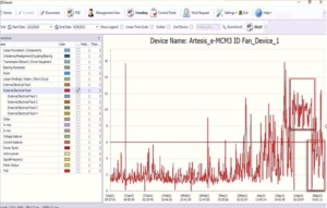
Figure 5.9 – Industrial examples where envelope analysis is the preferred diagnostic technique for some types of faults

5.10 Demodulation and Envelope Analysis – Synthesis

Envelope analysis represents one of the most important developments in condition monitoring of rotating machines. By separating the modulated information from the carrier vibration, transforms virtually invisible impacts into clearly identifiable diagnostic frequencies.

This capability explains its widespread adoption in modern FFT analyzers and continuous monitoring systems., Today, it is an indispensable tool for the early detection of defects in bearings and gears..

The following chapter will delve deeper into the advanced demodulation techniques, addressing the Hilbert Transform, a Kurtosis Espectral, o Fast Kurtogram, cyclostationary analysis and intelligent automatic filtering band selection algorithms, consolidating the link between the theory and practice of vibration diagnosis.

Demodulation and envelope analysis