Monitoring the operating cost of pumping groups
This article focuses on monitoring the operating cost of pumping groups based on the electric motor supply voltage and current..
1 INTRODUCTION
According to studies and industry guides, such as those from the Hydraulic Institute and Europump, the total life cycle cost of a pump over 10 a 20 years is made up of several categories, where electrical energy is, from afar, the largest component.
Typical percentages of costs over the life cycle of a pump are often distributed as follows:
- Electricity Costs (CE): 50% a 90% (the biggest slice, varying with pump size and use).
- Maintenance and Repair Costs (Cm): 10% a 25% (Some studies point to around 20% as an average).
- Initial Investment Cost (Cic): 5% a 15% (the purchase price of the pump and auxiliary equipment).
- Operation Costs (Co): 5% a 15% (supervisory staff, etc.).
- Installation and Start-up Costs (Cin): 5% a 10%.
The influence of pump efficiency (and the engine) in electricity consumption is enormous. Even small improvements in efficiency can result in substantial energy savings over time, given that pump sets operate many hours a day and have a long useful life. Therefore, the selection of efficient pumps, Operation at the point of best efficiency and adequate maintenance are crucial for optimizing operating costs.

Figure 1- Portions of the total life cycle cost of a pump over 10 a 20 years
2 – THE IMPORTANCE OF MONITORING THE PERFORMANCE OF PUMPING UNITS
The influence of pump efficiency on the motor's electrical energy consumption is direct and highly significant. The efficiency of a pump is a measure of its efficiency in converting the mechanical energy supplied by the engine into useful hydraulic energy. (fluid pressure and flow).
To understand this relationship, let's consider some key points:
- What is Pump Efficiency?
The yield (or efficiency) of a pump is the relationship between the hydraulic power output (useful power supplied to the fluid) and the mechanical input power (power supplied by the motor to the pump).
Pump Efficiency = (Output Hydraulic Power) / (Input Mechanical Power)
- Output Hydraulic Power: It is the energy that the pump effectively transmits to the fluid, manifested as flow and pressure.
- Input Mechanical Power: It is the energy that the motor supplies to the pump shaft.
- Where Energy is Lost?
No bomb is 100% efficient. Energy losses occur due to several factors:
- Hydraulic Losses: Caused by fluid friction on the internal surfaces of the pump (driving, desired) and turbulence.
- Volumetric Losses: Due to internal fluid leakage from the high pressure zone to the low pressure zone inside the pump.
- Mechanical Losses: Caused by friction in bearings, seals and other moving parts of the pump.
- The Relationship with the Electrical Energy Consumption of the Engine
The electric motor provides the mechanical power to the pump. The electrical energy consumed by the engine is converted into mechanical power, but also with their own losses (engine performance).
Electrical Power Consumed = (Pump Input Mechanical Power) / (Engine Efficiency)
Replacing the Pump Input Mechanical Power with the pump efficiency formula:
Electrical Power Consumed = (Output Hydraulic Power / Pump Efficiency) / (Engine Efficiency)
Simply put:
Electrical Power Consumed = Hydraulic Power Output / (Pump Efficiency × Motor Efficiency)
This formula clearly shows the influence:
- The lower the pump efficiency (and/or engine), the greater the electrical power consumed to provide the same output hydraulic power (that is, to pump the same flow rate at the same pressure).
- The higher the pump efficiency (and/or engine), The lower the electrical power consumed for the same useful work.
3 – LOSS OF PUMP EFFICIENCY
The loss of pump efficiency results from several factors:
- Component Wear: Lack of maintenance or inadequate maintenance leads to wear of key pump components, as drivers, wear rings, fencing, bearings and shafts.
- Impellers and Wear Rings: Wear on these components increases internal clearances and changes the designed geometries, allowing fluid to recirculate within the pump instead of being discharged. This results in hydraulic and volumetric losses, reducing pump efficiency. A pump with reduced efficiency requires more engine power to deliver the same flow and pressure, increasing energy consumption.
- Bearings and Seals: Worn or poorly lubricated bearings, and damaged seals, increase mechanical friction. This extra friction needs to be overcome by the engine, which translates into greater electrical energy consumption for the same hydraulic output.
- Deposit Accumulation: The accumulation of scale, sediment or other debris on the internal surfaces of the pump (impeller and volute) or in piping can reduce flow and increase resistance to flow. The pump must “work more” to overcome this additional resistance, resulting in higher energy consumption.
- Misalignment and Imbalance: Lack of preventive maintenance can lead to misalignment problems between the motor and the pump, or impeller imbalance. These problems generate excessive vibration and additional stress on components, increasing friction and mechanical losses. In addition to consuming more energy, also accelerate wear and tear and can lead to catastrophic failures.
4 – PUMP EFFICIENCY PARAMETERS
The efficiency of a pump is a measure of its efficiency in converting incoming mechanical energy (supplied by the engine) in useful hydraulic energy output (transferred to the fluid). To understand the parameters that affect this yield, It is essential to consider the following points:
- Caudal (Q):
- It is the volume of liquid that the pump is capable of displacing per unit of time, usually measured in cubic meters per hour (m³/h) or liters per minute (L/min). The flow rate is one of the main parameters that define the pump's operating point on its characteristic curve..
- Total Manometric Height (H):
- Also known as total head or pump pressure, represents the total energy that the pump adds to the fluid, measured in meters of liquid column (mcl) or pressure (Pascal, bar, psi). It is the pressure difference between the discharge and suction of the pump, considering static and dynamic heights (speed and friction).
- power (P):
- Hydraulic Power (Useful): It is the power effectively transmitted to the fluid, that is, the energy that the fluid gains. It is calculated from the flow rate and manometric head.
- Power in the shaft (Absorbed): It is the mechanical power supplied to the pump shaft by the motor.
- Electrical Power (Consumed): It is the power that the motor consumes from the electrical network to drive the pump.
- Rotation (N):
- The rotation speed of the rotor (RPM – revolutions per minute) directly affects the flow, the head and power of the pump. Changes in rotation modify the pump characteristic curve.
5 – THE CHARACTERISTICS CURVE OF A PUMP
The characteristic curve of a pump, also known as performance curve or pump curve, is a graph that shows the behavior of a hydraulic pump under different operating conditions. It is provided by the manufacturer and is essential for selecting the correct pump for a specific application and for understanding its performance in the system..

Figure 2 – Characteristic curves of a pump.
Normally, a pump characteristic curve presents several relationships on a single graph, with the flow(Q) in the horizontal shaft (came) and different parameters in the vertical vein (came Y):
- Manometric Height Curve (H) x Caudal (Q):
- This is the main and most important curve. It shows the total head (pressure) that the pump can generate for a given flow rate. Usually, as the heat increases, the head that the pump can provide decreases. The shape of this curve is crucial in determining the operating stability of the pump in different systems..
- Shaft Power Curve (P) x Caudal (Q):
- This curve indicates the mechanical power that the pump absorbs from the engine to operate at different flow rates.. It is essential to correctly size the motor that will drive the pump, ensuring it has sufficient power for all operating conditions, no overloads.
- Yield Curve (the) x Caudal (Q):
- Shows the efficiency of the pump in converting mechanical energy into useful hydraulic energy for each flow rate. Yield is expressed as a percentage (%). The Best Efficiency Point (BPE) ou Best Efficiency Point (BEP) is the point on the curve where the pump operates at its maximum efficiency, minimizing energy consumption and wear.
- Required NPSH Curve (NPSHr) x Caudal (Q):
- About NPSH (Net Positive Suction Head) is a critical parameter to avoid cavitation. The NPSHr curve indicates the minimum pressure required at the pump suction for it to operate without cavitation for a given flow rate.. It is vital to the design of the suction system, ensuring that the NPSH available in the system is always greater than the NPSH required by the pump.
The interpretation of the Characteristic Curve follows the following principles:
- Operating point: The pump operating point in a system is determined by the intersection of the pump characteristic curve and the system curve (which represents the pressure losses of the pipe and the static heights). It is at this point that the pump and system operate in balance.
- Pump selection: When selecting a pump, you should look for one that has your BPE (Best Efficiency Point) as close as possible to the desired operating point in your system. Operating the pump too far from the BPE can lead to low efficiency, higher energy consumption, vibrations and premature wear.
- Variations in rotor diameter: Many manufacturers provide multiple H x Q curves on the same graph for a single pump casing, but with different rotor diameters. This allows you to select the ideal rotor for the desired flow and head conditions..
- Variations in Rotation: Characteristic curves are plotted for a fixed rotation (RPM). If the pump rotation is changed (for example, with a frequency inverter), pump performance will change, and new curves would be needed or calculated based on affinity laws.
6 – THE AFFINITY LAWS OF CENTRIFUGAL PUMPS
The Affinity Laws of centrifugal pumps are a set of mathematical relationships that describe how a pump performs (caudal, head and power) changes when there are changes in its rotation speed (RPM) or rotor diameter. They allow the behavior of a pump to be predicted without the need for extensive testing for each operating condition..
The main objective of the Affinity Laws is to optimize the functioning of the pump and hydraulic system, allowing:
- Performance Tuning: Predict pump performance at different rotational speeds (for example, when using a frequency inverter) or with rotors of slightly different diameters, without having to consult a specific characteristic curve for each scenario.
- Energy efficiency: Identify the most efficient operating conditions, helping to reduce energy consumption.
- Sizing and selection: Assist in pump selection and motor sizing, ensuring the pump meets the needs of the system with maximum efficiency.
- Scenario simulation: Simulate the impact of changes to pump or system specifications.
Affinity laws are applicable to geometrically similar pumps and assume that pump efficiency remains constant between operating conditions.. Although this last premise is not 100% accurate in all variations (especially for large RPM or diameter changes), it offers a very good approximation for most practical applications. The relationships are as follows:
For changes in rotation speed (N), maintaining rotor diameter (D) constant:
- Caudal (Q) and Rotation (N):
The FLOW is directly proportional to rotation.

- Manometric Height (H) and Rotation (N):
The head is directly proportional to the square of the rotation.

- power (P) and Rotation (N):
The absorbed power is directly proportional to the cube of rotation.

7 – THE DIGITAL TWIN OF THE ELECTRIC MOTOR
In 1992 the article was published[i] in which the result of work developed for NASA was presented, in which the electric motor was mathematically modeled as a transfer function between the voltage and current supplying the motor, allowing the construction of the digital twin, what is, therefore, a matrix.

Figure 3 – The mathematical modeling of an AC electric motor
This means that, from monitoring the voltage and current and power supply to the motor,, in the three phases, you can build your digital twin and, from the deviations from the initial model, determine its operating condition.

Figure 4 – Monitoring the engine condition through comparison with the digital twin
This technology was commercialized by ARTESIS and is currently standardized in ISO 20958 – electrical signature analysis of three phase induction motors.
8 – MONITORING PUMP PERFORMANCE THROUGH ELECTRICAL SIGNATURE
The monitor e-MCM (Electrical Motor Condition Monitor) processes voltage and current signals to extract critical performance metrics. Flow and pressure estimation is performed using proprietary algorithms that convert electrical data into accurate flow and pressure readings, no need for traditional sensors. Pump curves are generated in real time, allowing pump efficiency to be dynamically viewed and compared to BEP for instant operational adjustments.. Furthermore, it allows the detection of faults such as cavitation, imbalances and mechanical wear through unique electrical signature patterns.

Figure 5 – Monitoring graphs, In real time, pump performance, through the electrical signature of the motor in which you can see the point at which the pump is working and the evolution of flow and power.
The main functionalities provided by this technology are:
- Sensorless performance metrics: Monitor a caudal, pressure and efficiency in real time with greater accuracy than 95%.
- Optional sensor integration: Can combine data from real sensors, if available, to increase accuracy and redundancy.
- Real-time alerts: Instant notifications for efficiency drops, mechanical failures and hazardous conditions.
- Power Analysis Tools: Quantifies energy consumption and identifies oversized pumps.
- Power curve visualization: Monitors flow to power relationships to maintain maximum efficiency.
- Historical trend analysis: You can access annual and performance reports 24 hours to optimize operating time in flow zones.
- Annual flow distribution: Shows operating time in different flow zones. Reveals efficient or inefficient functioning.
9 – MONITORING THE PERFORMANCE OF THE PUMPING GROUP THROUGH THE ELECTRICAL SIGNATURE
Example 1
No artigo LNG Carrier Seawater Pump Condition Monitoring[ii] an example of its application to a ship's pump is presented.
In it you can see several graphs with an application of the evolution of the electrical parameters associated with the degradation of the operating condition of the pump impeller.

Figure 6 – Trend graph showing a gradual and progressive decrease in the active power and power factor parameters for the main cooling seawater pump number 1.

Figure 7 – Internal pump components after removal for inspection. Note significant metal loss from body flow vane tips (fins). About 19 mm of metal were lost in two places. The thickness of the fins was also reduced from the original dimension of 7 mm for 4,5 mm. It was found that the anomaly in the blade passage was caused by this damage, and not due to deterioration of the impeller.

Figure 8 – After disassembly, It was discovered that erosion had produced a hole in the pump body, at the point where a wear ring retaining screw caused a localized flow disturbance.
Example 2
The energy audit at the mine revealed many pumps operating with low efficiency. High energy losses were identified. The user wanted to continuously monitor the performance and efficiency of the pump. Like this, a method was needed to monitor mechanical and electrical failures through a single system.
It was decided to monitor the Electrical Signal of the motor supply as it allows performance to be monitored directly from the motor control panel using the MCM technique.. This eliminates the need for separate flow/pressure sensors and provides a unified view by combining mechanical condition, electrical and pump performance monitoring. Below you can see a photograph of the system installed in the engine cabinet.

Figure 9 – Installation of the monitoring system on the engine electrical panel
The characteristics of the pump were as follows:
- Process Water Pump
- Model: 150QC-DWU
- Motor power: 110 kW
- 1480 rpm nominal; 1630 rpm (with straps)
- Polis/Belts add ~2% energy loss

Figure 10 – Photography of the pumping group
From monitoring it is concluded:
- Frequent operation outside the BEP
The point of best efficiency (BEP) is where the pump achieves maximum efficiency with minimum energy consumption.
Documentation and field measurements show that this pump model 150QC-DWU often operates far from its BEP, particularly in low flow and high pressure conditions.
- Belt and pulley transmission system
Rated engine speed of ~1490 rpm (4 poles) is increased to ~1630 rpm on the pump shaft using a belt and pulley arrangement.
In addition to the inefficiencies inherent to the pump, This configuration introduces up to 2% additional transmission losses.
- Low efficiency and low flow risks
Low efficiency: Operating outside the ideal operating range increases energy costs and reduces performance. Potential causes include wear, incorrect sizing or inadequate maintenance.
Low flow: the actual flow is below project expectations, at risk of overheating, cavitation and substandard performance.
- High temperature risk
High operating or fluid temperatures can damage seals, bearings and other internal components, leading to frequent maintenance or failures.
- Flow irregularities and cavitation
eMCM's model-based fault detection reveals broadband noise near the 50 Hz, indicating flow instability — often related to low-flow operation.
Prolonged low-flow conditions increase the risk of cavitation, which reduces the mechanical useful life in the medium term.
In general, the tendency of the pump to operate at low flow rate and high pressure significantly increases the probability of inefficiency, cavitation and mechanical wear, emphasizing the need for better adaptation of the pump to real operating conditions and continuous monitoring of performance.
Below you can see one of the graphs obtained from the system showing the statistical distribution of the flow rates at which the pump operated.

Figure 11- Statistical distribution of flow rates at which the pump operated.
Below you can see a histogram. This histogram illustrates the percentage of operating time spent at various flow rates over the course of a week. On the horizontal axis, can see the flow rate in cubic meters per hour (m³/h), while the vertical axis represents the percentage of total operating time in each flow interval.

Figure 12 – Histogram illustrating the percentage of operating time spent at various flow rates over the course of a week.
Comments on this histogram are presented below:
Color-coded regions
- Light yellow (inefficient zone): The majority of pump operating time falls within this range, indicating that the pump is operating well below the flow rate for which it was designed, consuming excess energy and operating inefficiently.
- Verde (efficient zone): About 280–500 m³/h. A very short operating time is shown here, meaning the pump rarely reaches the operating range where it would achieve the best energy efficiency.
- Rosa (high flow, risk zone): Represents very high flow rates. The histogram shows almost no activity in this zone, therefore the pump essentially never operates in these extreme flow conditions.
BEP (point of best efficiency)
Marked by the red dashed line in 421,5 m³/h, is where the pump would theoretically achieve ideal efficiency. The histogram reveals that the pump almost never operates close to this point, confirming a large difference between actual and ideal operating conditions.
Dominant flow range
The flow values between 90 e 110 m³/h dominate the histogram, meaning the pump is consistently operating at a fraction of its intended flow capacity. This misalignment not only increases energy consumption, but it can also lead to long-term mechanical problems.
In general, the chart highlights a significant opportunity to improve performance: By adjusting or replacing the pump — or by modifying the system to better match the pump's design parameters — the installation could potentially save energy, reduce equipment wear and tear and operate closer to the point of best efficiency.
Flow irregularities and cavitation
eMCM model-based fault detection reveals broadband noise near the sidebands of 50 Hz, indicating flow instability — often related to low-flow operation.

Figure 13 – Supply current analysis spectra
Prolonged low-flow conditions increase the risk of cavitation, which reduces the mechanical useful life in the medium term.
In general, the tendency of the pump to operate at low flow and high pressure significantly increases the likelihood of inefficiency, cavitation and mechanical wear, emphasizing the need for better adaptation of the pump to real operating conditions and continuous monitoring of performance.
The summary of the problems observed was as follows:
- Operation mainly in low flow/high pressure conditions
- Longe do BEP, leading to low efficiency (40–60%).
- Cavitation and mechanical stress.

Figure 14 – Summary of observed problems
The recommended actions were as follows:
Alternative pump selection (Model: “XXX”)
- Caudal nominal: ~215 m³/h
- Rated power: 55 kW
- Efficiency: ~81,3% a BEP
- Expected reduction in energy consumption: ~56.6%
In the following figure, the proposed new pump model is analyzed, which can significantly increase overall efficiency and reduce energy costs.

Figure 15 – Characteristic curve of the proposed new pump model
Why a new pump? The current configuration often works far from its best efficiency point, causing high energy consumption and additional mechanical wear. A more appropriately sized pump will better match actual flow and pressure needs, improving both performance and reliability.
- Proposed model XXX
- Caudal nominal: 215 m³/h
- Rated power consumption: 55 kW
- Efficiency: near 81,3% at the point of best efficiency
- Expected energy savings: up until 56,6% less power consumption compared to our current setup
Main advantages
- Better adaptation to operating conditions: operating close to design flow and head means less energy wastage.
- Reduced operating costs: Greater efficiency will significantly reduce annual energy bills.
- Less mechanical wear: Working in your ideal range extends component life and reduces the need for frequent maintenance.
Next steps
- Conduct a detailed cost-benefit analysis, including return on investment.
- It will also consider installation logistics, the compatibility of materials and whether the addition of a frequency inverter (VFD) could provide more energy savings.
By switching to this new, more efficient model, can resolve pump operating issues outside of its ideal operating range and drastically reduce energy consumption and maintenance costs.
The expected return on investment period is 1,28 years.
| Current power consumption (kWh/year) | 602,880 |
| Proposed power consumption (kWh/year) | 264,707 |
| Annual Energy Savings (kWh) | 338,173 |
| Annual Cost Savings (USD) | $ 30,435.57 |
| New pump investment cost (USD) | $ 39,000.00 |
| ROI (%) | 78% |
| Investment payback period (Years) | 1.28 |
The results of the measurements carried out by the system were then validated with on-site instrumentation..

Figure 16 – Comparison between flow measured with a flowmeter and by the eMCM system
The blue line represents the flow measured with a flow meter and the orange line represents the flow estimate from the eMCM.
We can see that, under normal operating conditions, the lines follow each other.
Side-by-side comparison of flow sensor data and eMCM estimated flow, concludes:
- Consistent trend alignment and near overlap in normal trading ranges
- Overall deviation of around ±3% confirms high accuracy
- Demonstrates reliable real-time monitoring without additional flow sensors
11 – CONCLUSION
Here we presented an innovative sensorless pump performance monitoring solution, leveraging Electrical Signature Analysis technology (ESA). When analyzing voltage and current data, the system provides real-time information about the flow, the pressure and condition of the pump and motor – eliminating the need for physical sensors. This innovation allows companies to optimize operations, reduce costs and increase sustainability by monitoring the operating cost of pumping groups.
REFERENCES
- [i]Fault diagnosis for the Space Shuttle main engine, Ahmet Sensing; Journal of Guidance Control and Dynamics 15(2) · May 1992
- [ii] LNG Carrier Seawater Pump Condition Monitoring, Geoff Walker, ORBIT Vol.31 No.1 2011