Vibration analyzer 5 - the Windows

Vibration analyzer 5 – the Windows

Then, on vibration analyzer 5, we present the theme of the windows in the waveform (“Windows”), when they take place how they are carried out with a vibration analyzer. Like this, this article is part of a series of articles that explain how a vibration analyzer works. When we do Vibration Analysis, we need to understand how an analyzer works. Therefore, here we present the concepts of digital signal analysis, implemented in an FFT analyzer. In order to be easy to understand, we always present them from the user's point of view, in a vibration analyzer when performing predictive maintenance. Then, no link, we can see a range of Vibration analyzers provided by D4VIB. Then, in Vibration Analyzer 5, we present the content of this series of articles.

- Introduction

5 Vibration analyzer 5 – The implementation of windows in the waveform (windows)

5.1 The need for windows

parallel, to what was previously said about aliasing, there is another FFT property, that affects its use in frequency domain analysis. let's remember, that the FFT calculates the frequency spectrum, from a set of samples from the entry, designated a block of time.

5.1.1 What happens when the waveform is periodic in the time block

To begin, it is worth mentioning, that the FFT is based on the assumption that the time block, is repeated over time.

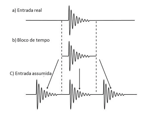
In order to illustrate or text this figure is here. Like this, here we see Figure 5.1. As mentioned in the FFT, part of the principle, that the time block / waveform, is repeated over time. — Figure 5.1. As mentioned in the FFT, part of the principle, that the time block / waveform, is repeated over time.

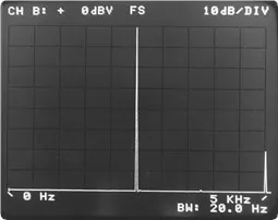
De facto, with the transient vibration, of the previous figure, this does not cause any problems. On the other hand, what happens if you are measuring a continuous signal? Take for example the case that we are measuring a wave of a sine. Let's look at the situation where the block of time contains an integer number of sine wave cycles. So in this case the block of time is repeated indefinitely, and it is de facto, real wave. Like this, in this case, the input waveform is periodic in the time block.

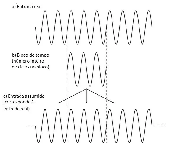
In order to illustrate the text this figure is in here. Like this, here we see Figure 5.2. As it was seen, in this situation the input signal is periodic in the time block. — Figure 5.2. As it was seen, in this situation the input signal is periodic in the time block.

5.1.2 What happens when the non-periodic waveform in the time block

On the contrary, when the entry is not periodic in the time block, the figure below, shows the difficulty with this assumption. In this situation, the FFT is calculated based on the highly distorted waveform that we see in c).

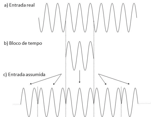
In order to illustrate or text this figure is emaqui. Like this, here we see Figure 5.3 Non-periodic input signal in the time block — Figure 5.3. As mentioned, in this figure we see the non-periodic waveform in the time block.

5.1.3 What are the escapes

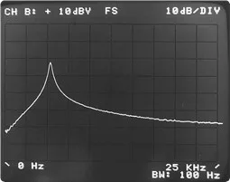
We know that when the waveform is a sine, the frequency spectrum has a single line. On the contrary, we know that abrupt phenomena in a domain, are spread across the other domain. Then, in the figure 5.4 we see that these considerations are correct to a real extent. In the figures a) & b), you see a waveform that is periodic in the time block. Like this, its frequency spectrum is a single line whose width is determined only by the resolution of our analyzer. On the other hand, nas figuras c) and d) we see a sinusoidal waveform that is not periodic in the time block. As predicted, its energy was spread across the spectrum, . a) e b) – when they take place) and d) – Non-periodic sine wave in the time block

In order to illustrate or text this figure is here. Like this, here we see Figure 26 Actual results of the FFT transform a) e b) Periodic sinuous wave in the time block — a) e b) – Waveform is periodic in the time block

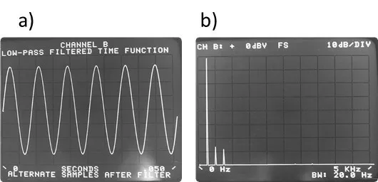
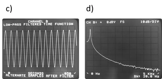
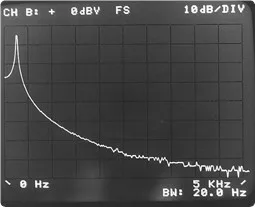
In order to illustrate or text this figure is here. Like this, here we see Figure 5.4 Real results of the FFTc transform) and d) Non-periodic sine wave in the time block — c) e b) Non-periodic waveform in the time block. Figure 5.4. As mentioned, in these figures we can see the real results of the FFT, when the waveform is periodic and not periodic, in the time block.

Like this, this scattering of energy, across all frequency domains, It is known as escape (leakage). actually, as the name implies, we see energy leaks, of a spectrum line, for all other lines.

5.1.4 Leaks result?

It has to be seen that, the energy leaks are due to the fact of having a finite block of time. De facto, so that a sine wave has a single line spectrum, it must exist forever, from less infinite to more infinite. If you had an infinite block of time, the FFT would calculate the correct spectrum, with a single line. However, a finite time record of the sine wave is only observed because we are not willing to wait forever, to measure a spectrum. Like this, this can cause leakage if continuous input is not periodic, in the time block. Is obvious, from the observation of Figure 5.4, that the leakage problem is serious enough to completely mask small signs, close to the largest sine waves. In these circumstances, the FFT frequency spectrum calculation algorithm does not provide a useful vibration analyzer.

5.2 Avibration analyzer 5 – What are “windows”?

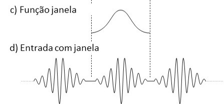
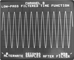
In order to solve this problem, to follow, in Vibration Analyzer 5, let's see how a solution known as “windows” is implemented( “Windows” in English). In the figure 5.5 ( a e b) we reproduce the input waveform of a sine that is not periodic in the time block. In this case, we noticed that most of the problem seems to be on both sides of the time block. De facto, in the present situation the center is a sine wave, well represented. Like this, if the FFT could ignore the ends and focus on the middle of the time block, one would expect to be much closer to the single line spectrum, which is correct. For example, if we multiply the block of time by a function, which is zero at the ends of the block and large in the middle, the result of calculating the FFT would be mainly from the middle of the time block. In the figure 5.5 c) we see one of these functions. The name of these functions is “window functions”. These functions effectively force you to look at the data, through a narrow window.

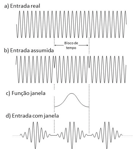
In order to illustrate the text, this figure is in Vibration Analyzer 5. Like this, here we see Figure 5.5 The effect of the window on the time domain. — Figure 5.5. – As mentioned, you c) and d), we see a “window function” and its effect on the waveform that will be used to calculate the FFT.

5.3 The effect of the window function

Effectively the Figure 5.6, shows the great improvement that has been obtained by applying windows to data that are not periodic in the time block. However, it is important to realize that the input data has been tampered with and we cannot expect perfect results. Next on Vibration Analyzer 5, let's see this question. The FFT assumes that the waveform looks like the Figure 5.5 d). In other words, the FFT assumes the waveform as a sine of modulated amplitude. This generates a frequency spectrum, which is closer to the correct line of the sine input wave than Figure 5.5 b), but it is still not correct. De facto, a Figure 5.6 c) shows that data with windows does not have a spectrum with such a narrow line, how much a function, without window, which is periodic in the time block.

In order to illustrate the text, this figure is in Vibration Analyzer 5. Like this, here we see figure a) Non-periodic sine wave in the time block — a) Non-periodic sine wave within the time sample block

In order to illustrate the text, this figure is in Vibration Analyzer 5. Like this, here we see the figure 28 b) Resulting FFT without window function — b) Resulting FFT without window function

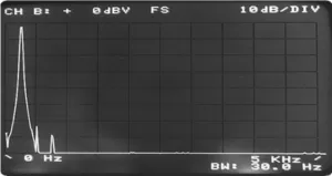
In order to illustrate the text, this figure is in Vibration Analyzer 5. Like this, here we see the figure 28 c) FFT results with a window function — c) FFT results with a Figure window function 5.6. Leakage reduction using windows in the time block

5.4 A janela Hanning

There are many functions that can be used to implement windows on samples in the waveform. Next on Vibration Analyzer 5, let's see this the types of windows. De facto, the most common one is called Hanning. The Hanning window was used in Figure 5.7, as an example of leakage reduction with windows. The Hanning window is also commonly used when measuring vibrations with random noise. For example, this is the case for the stationary vibrations that we measure on machines.

In order to illustrate the text, this figure is in Vibration Analyzer 5. Like this, here we see the figure 29 a) Leak-free measurement - periodic entry in the time block — a) Leak-free measurement – periodic entry in the time block

b) Measurement with window – non-periodic entry in the time block

In order to illustrate the text, this figure is in Vibration Analyzer 5. Like this, here we see the figure 29 b) Measurement with window - non-periodic entry in the time block — b) Measurement with window – non-periodic entry in the time block

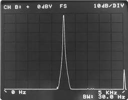
Figure 5.7. The window function reduces leakage, but does not eliminate them

5.5 The uniform window (also called rectangular)

5.5.1 A limitation of the Hanning window

It was seen that the Hanning window does an acceptably good job in the sine wave examples, both periodic and non-periodic in the time register. If this is true, why use other windows? Suppose that, instead of wanting the frequency spectrum of a continuous signal, if you would like to get a spectrum for a transient event. To this end, in the figure 5.8 a) we show a typical transient vibration. If it multiplies by the function of the window in the figure 5.8 b), you would get the highly distorted signal shown in the figure 5.8 c).

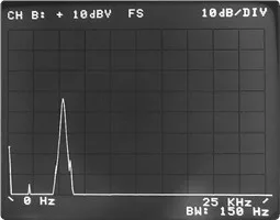In order to illustrate the text, this figure is in Vibration Analyzer 5. Like this, here we see Figure 5.8 The windows function loses information about transient events — Figure 5.8 As mentioned here we see that the Hanning window function, loses information on transient events.

The frequency spectrum of a real transient with and without the Hanning window is shown in Figure 5.9. Hanning's window transformed the transient. It is, which has energy spread widely across the frequency domain, it looked more like a sine wave. Therefore, we can see that for transient phenomena we don't want to use the Hanning window.

5.5.2 The Uniform window

We would like to use all the data in the time block equally or evenly. Hence if you use the uniform window that weighs the entire block of time equally.

In order to illustrate the text, this figure is in Vibration Analyzer 5. Like this, here we see the figure 31 a) Transient vibration spectrum without window — a) Without window – Transient vibration spectrum without window

b) Janela Hanning – Transient vibration spectrum with Hanning window

In order to illustrate the text, this figure is in Vibration Analyzer 5. Like this, here we see figure b) Transient vibration spectrum with Hanning window — b) Janela Hanning – Transient vibration spectrum with Hanning window

Figure 5.9 Transient vibration spectra, with and without Hanning window.

What referred to the uniform window in the analysis of transient vibrations can be generalized. Note that the transient has the property of having a value of zero at the beginning and end of the time block. Remember that windows were introduced to force the entry to be zero at the ends of the block of time. In this case, there is no need to use the window at the entrance.

5.6 Auto-window signs

Any sign like this, is called an “auto-window”, because it does not require a window. This is effectively so, because it occurs completely within a block of time. These signals do not generate leaks in the FFT and therefore do not need a window. There are many examples of "auto-window" signs, some of which we show in Figure 5.10. The frequency analysis of the following signals can be done without a window, due to the fact that they are auto-window signs:

Impacts,
Impulses,
Shock responses,
Sine bursts, noise or impulses
Pseudo-random noise

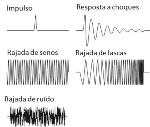
In order to illustrate the text, this figure is in Vibration Analyzer 5. Like this, here we see Figure 32 Examples of auto window function — Figure 5.10. In this figure we see examples of auto-window signals.

5.7 The flat top window “Flat Top”

Previously we saw that a uniform window is needed, to analyze auto-window functions, such as the example of transient vibrations. Besides that, we need a Hanning window to measure noise and periodic signals, as sine waves. It is now necessary to introduce a third window function. So now we introduce, a flat top window, to avoid a Hanning window effect.

5.7.1 Hanning window limitations

To understand this effect, you need to look at the Hanning window in the frequency domain. Remember that the FFT acts as a set of parallel filters. To figure 5.11 shows the shape of those filters, when using Hanning window. We can see that the Hanning function gives the filter, a very rounded top. In this situation if a frequency component of the analyzed signal, fall in the center in the filter, your level will be accurately measured. Otherwise, the shape of the filter will attenuate the component until 1,5 dB (16%), when it falls in the middle of the gap between the filters.

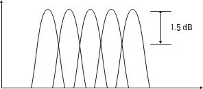
In order to illustrate or text this figure is here. Like this, here we see Figure 5.11 Hanning bandpass filter window shape — Figure 5.11. – In this figure we see how the Hanning window attenuates the amplitude of the frequency component.

De facto, when trying to measure the amplitude of a signal, with accuracy, this error is very big.

5.7.2 The measurement accuracy of the flat top window

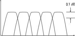
So we have that the solution to this problem, is to choose a window function that gives the filter a flatter top. In the figure 5.12 this flatter top shape is shown. actually, the amplitude error of this window does not exceed 0,1 dB (1%). That way, measurement accuracy, we got an improvement of 1,4 dB.

In order to illustrate the text this figure is in here. Like this, here we see Figure 5.12 Shape of the flat top window — Figure 5.12. – As mentioned in this figure we see the shape of the flat top window.

5.7.3 The resolution reduction of the flat top window

It should be noted that improving the accuracy in measuring the level, does not come without a price. To figure 5.15 shows that the top of the window has been flattened, at the expense of widening the filter skirts. Therefore, we lost some resolution capacity and the ability to observe a small component, close to a large. Some vibration analyzers offer commands and functions from the “flat-top” window. In this way we can choose between increased accuracy for balancing work, for example, or frequency resolution, enhanced, from the “Hanning” window.

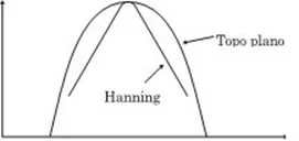
In order to illustrate the text this figure is in here. Like this, here we see Figure 5.13 Reduced resolution of the flat top window — Figure 5.13. As mentioned, in this figure we see the reduced resolution of the flat top window

5.8 Vibration analyzer 5 – Other window functions

There are many other window functions, but the three listed above are the most common for general measures. However, for special situations of the measure, other groups of window functions may be useful. The following are two windows that are particularly useful, when measuring the frequency response of mechanical structures, through impact tests.

5.8.1 Impact test – the windows of strength and response

An instrumented hammer is often used, to impact a structure and make it vibrate at its natural frequency. To measure the strength of the impact, on top of the hammer impact head, a force transducer is placed. Thus instrumented hammers are used for determining natural frequencies and measuring frequency response. Normally, the power input is connected to an analyzer channel and the structure response, measured with an accelerometer, is connected to another channel. This impact of force is obviously an auto-window function. The response of the structure is also auto-window. This is in fact so if the signal disappears within the analyzer time block.

5.8.2 The response window

In order to ensure that the response goes to zero by the end of the time block, sometimes an exponential window is added. Like this, this window is called the response window. Figure A 5.14 shows a response window, acting on the response of a weakly damped structure. Due to the structure being poorly cushioned, the vibration did not fully decline until the end of the time block. Notice-i know, unlike the Hanning window, the response window value is not zero, at both ends of the time block. It is known that the response of the structure will be zero at the beginning of the time block (before the hammer hit). Seen this, there is no need for the window function to be zero. Besides that, we know that most of the information about the structural response, is contained at the beginning of the time block. So, it is necessary to ensure that this area, be more taken into account, by the response window function.

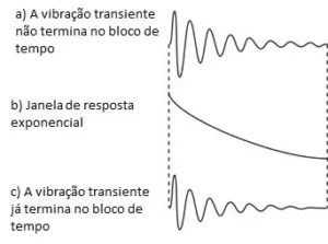
In order to illustrate the text this figure is in here. Like this, here we see Figure 36 - Using the exponential response window — Figure 5.14. As mentioned, in this figure, we see how to use the exponential window.

5.8.3 The strength window

The time block of the exciting force, should only be the impact signal with the structure. However, the movement of the hammer before and after hitting the structure, can cause noise in the time block. To avoid this we use a power window. Like this, we can see this in Figure 5.15. The force window has a value equal to the unit, where impact data is valid and zero everywhere else. This is effectively so, so that the analyzer does not measure any noise, that can be present.

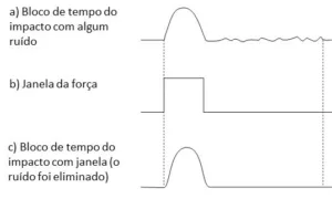
In order to illustrate the text this figure is in here. Like this, here we see Figure 5.15 - Using the force window — Figure 5.15. – As mentioned in this figure, we see how the force window is used.

5.9 – Bandpass filter forms or window functions?

As previously mentioned, sometimes referred to window functions in the time domain. On other occasions, the theme was referred to using the reference to the form of bandpass filters in the frequency domain, caused by these windows. In both situations the perspective was freely changed to the domain that produces the simplest explanation. Similarly, some vibration analyzers call windows uniform, hanning e flat-top “windows” and other analyzers call these functions “forms pass band”. In fact we use the terminology that is easiest for the problem at hand. This is because they are completely interchangeable. In the same way, the time and frequency domains are completely equivalent. For example in the specification of the vibration analyzer ADASH 4500VA it refers to having the following windows: Rectangular, Hanning, Exponential, Transient.

Vibration analyzer 5 – the Windows

Vibration analyzer 5 – the Windows