Vibration data processing

Introduction – Vibration data processing

Vibration data processing is the subject of this chapter.. This concerns the configuration and limitations of the instrumentation used to make routine vibration measurements.. Included are FFT analyzers (Fast Fourier Transform Analyzers) and data collectors. FFT analyzer and data logger are used to view the waveform (to evaluate periods and orbits), in spectral analysis and time waveform evaluation. The time waveform is used to screen and analyze its shape..

Vibration data processing and waveform display (oscilloscope)

Waveform display measures and displays voltages that vary with time. A transducer converts the mechanical vibration into a calibrated proportional electrical signal in engineering units. (UE) milivolts (mv) per micrometer (μm), millimeters per second (mm/s) or g.

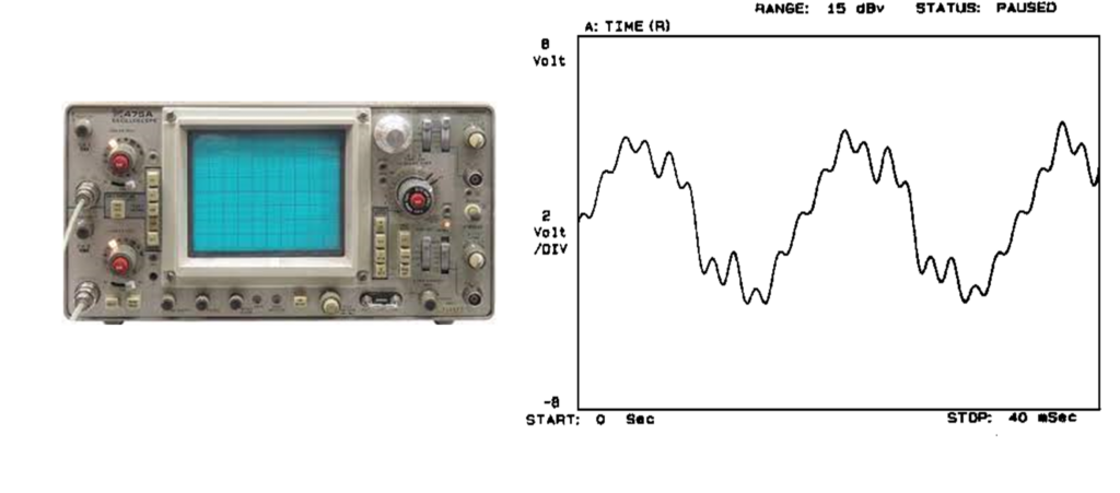
Waveform screens are used to show waveforms in time, orbits and markers related to events such as shaft rotation as seen in the following figure.

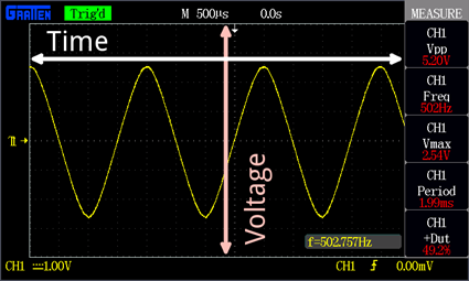
the function of trigger

the function of trigger (kitten) is an important function of both the oscilloscope and the FFT analyzer. A device of trigger starts data acquisition at a specific time or amplitude and controls data acquisition through a specific signal (vibration or trigger). The oscilloscope can be placed in trigger automatic to continuously sample the data. Triggering can be done on a selected signal based on voltage slope and/or magnitude. The oscilloscope can be configured to make a single measurement triggered at a specific voltage. For continuous measurements, an optical pickup or a proximity sensor can be used as a triggers continuous, at the frequency of the shaft.

Input external intensity

A controlled blanking or intensity mark can be displayed on the oscilloscope screen, through the application of a +/- 5back to z-shaft connector. Input can be AC ​​coupled (i.e., no DC passes). If you are not, a condenser with proximity sensors with more than 5 volts DC. The z-shaft suppression is used to measure phase and to relate a mark on the shaft to vibration during balancing. The suppression signal is obtained from the trigger from a proximity or optical sensor.

Vibration data processing and the FFT analyzer

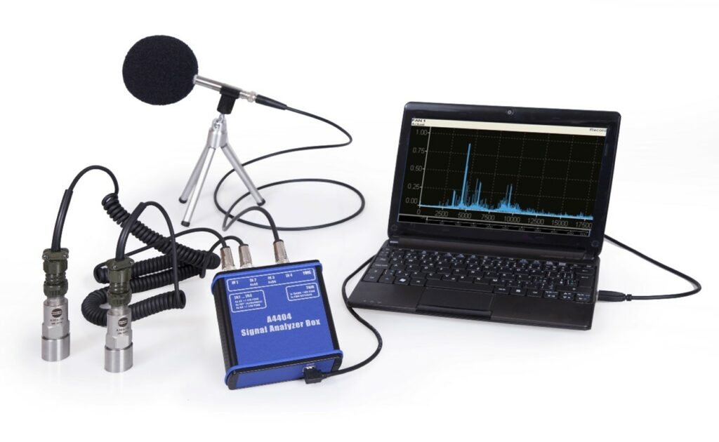
FFT analyzer is a digital instrument.

Analog signal conversion into a sample set

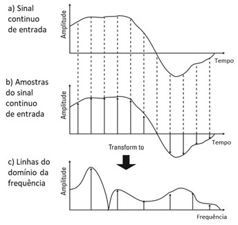
A block of data digitized in an analog-to-digital converter is processed in a fast Fourier transform algorithm (FFT) to produce a spectrum.

The time waveform is reconstructed from the digitized data block. A two-channel FFT analyzer allows obtaining the properties of and phase between two obtained signals. the analyzer, de FFT, has a high resolution, but may compromise the accuracy of the range, depending on your setup. It is basically a parser to use on steady state rather than transient data..

The analyzer collects a block of data at a high sampling rate – eg.: superior a 200000 samples per second – depending on the highest frequency range of the analyzer. The parser requires a complete block of an entire cycle before processing any data by the FFT.

This means that, for low frequencies (less than 10 Hz), long sampling times are required before FFT processing starts. The analyzer's ability to monitor events when the speed is changing rapidly is, therefore, committed.

At common machine frequencies, the calculation time for processing the FFT, is a fraction of the data acquisition and automatic time variation time.

To learn more about this topic click here.

O zoom

A zoom function in the FFT analyzer increases the resolution; are used 400 or 800 lines, but the frequency range is decreased to a defined frequency (beginning or center) to achieve a frequency resolution. Resolution refers to the instrument's ability to see frequencies that are very close together in the spectrum..

FFT analyzers have windows to prepare scanned data for the FFT process. The dynamic range of FFT parsers is, currently, close to 120dB (24 bits). Therefore, a signal with one millivolt can be resolved in the presence of a two-volt signal. The many other features of FFT analyzers include orbits, bodé curves, polar charts, waterfall diagrams, and real and imaginary graphs used for modal analysis.

Vibration data processing and the data collector

the data collector, which nowadays is also a FF parserT, collects and stores selected vibration parameters, like the global vibration, total vibration in selected frequency bands, spectral, waveforms in time, orbits, waterfall diagrams, high frequency measurements and envelope spectra.

In a pre-established inspection routine the overall level of vibrations is usually stored as vibration speed, in peak or rms, and related to measuring points, which may include many machines.

Data is transferred to computer, to compare them with previously acquired information, for what, any changes in machine condition, can be identified.

FFT algorithms were introduced in the collectors and, after several generations, many are now respectable FFT analyzers with adequate resolution and dynamic range. Some collectors have capacity for more than 6400 lines. Obviously, data acquisition time increases 16 times more than that of a spectrum of 400 lines.

Typically available line numbers are 100, 200, 400, 800, 1600, 3200 e 6400. The high number of rows provides a valid magnification, but expansion is needed to see data very close on the computer screen.

Vibration data processing and No. of samples in the time block and No. of lines in the spectrum

The input signal from a transducer is digitized before processing by FFT, as shown in the picture. The number of samples stored in the input memory (buffers) of the analyzers depends on the number of lines selected for the spectrum. The input memory records these values ​​as components Y (amplitude) e X (time) equally spaced.

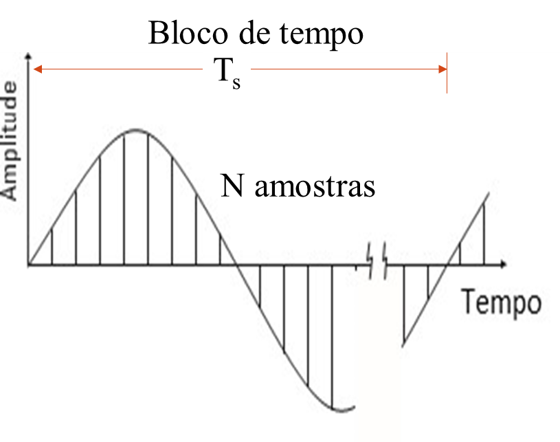
No frequency less than 1/T can be identified_s, because the information in the parser buffer would be incomplete.

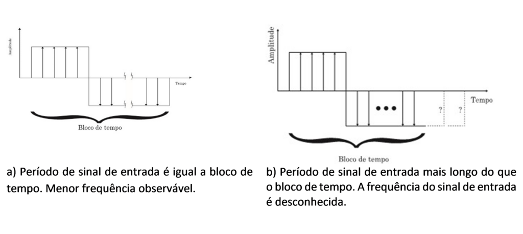
The following shows the relationship between the number of samples in the time block and the number of lines in the spectrum..

The following figure shows the result of transforming the waveform samples, equally spaced, on a spectrum of 100 lines or bins. Are bins equally spaced start at lowest resolvable frequency, which is one divided by the sampling time, that is, 1/T_s. In this case, how do you have a frequency gram of 100 Hz, and the number of lines is 100, there is a resolution of 1 Hz. the inverse of 1 Hz is a second that corresponds to the acquisition time of a block of time to calculate the FFT and obtain this spectrum.

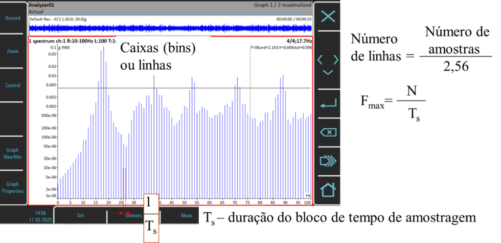
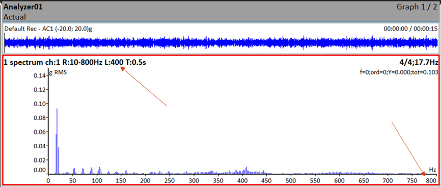
The spectrum can have N bins (lines) – normally of 100 a 6400, depending on the number of samples collected by the analyzer or data collector. The number of samples in the time block is 1024, if you intend 400 lines in the spectrum.

To adjust the number of samples collected over the data acquisition time, digital filtering is used.. The number of time block samples is, therefore, related to the number of lines selected for the spectrum, by a factor of 2,56.

The data sampling rate over time, is adjusted by the analyzer, to obtain the required number of samples over the duration of the selected data collection time (N/F_max).

The formula for maximum frequency and data acquisition time is F_max = N/data collection time. The value of F_max is placed in the analyzer, and the time display automatically has the appropriate period, as seen in the figure below.

For example, if the value of F_max is 800 Hz; and the number of lines is 400, it follows that, the data collection time must be T_s = N/F_max = 400/800, or 0,5 seconds. This relationship establishes the time interval necessary to collect the data., regardless of the speed of the measuring equipment.

Vibration data processing and aliasing

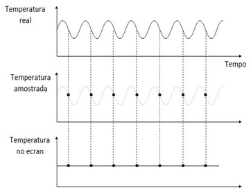
Sampling the waveform at an insufficient rate shown in the figure results in lost data and causes false frequencies due to the aliasing. This phenomenon occurs in the spectrum, if the sampling rate is less than the frequencies present in the data.

The in the following figure (topo) shows a sampling of data at the same frequency as a temperature varies. The resulting scanned data would be a straight line. false frequencies or aliased are obtained in the spectrum when the sampling frequency is less than the highest frequency present in the data.

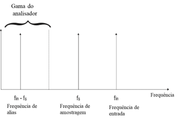
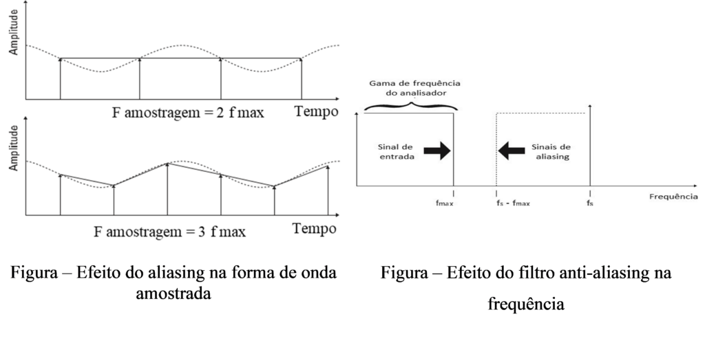
Therefore, be careful with FFT algorithms that have no filters anti-aliasing. The Nyquist Criterion says that the sample rate of an analyzer must be greater than twice the highest frequency present.. At the moment, the equipment provided as frequency analyzers, have all filters of this type, so your users don't have to worry about it.

The following figure illustrates the effect of a sampling frequency of two and three times the maximum frequency.. the filter anti-aliasing is a low-pass filter that eliminates frequencies in the data that are high enough to cause aliasing.

In the following video, see an example of aliasing. The frequency of the filmed image is almost equal to the speed of rotation of the helicopter's rotor and therefore the propeller appears to be almost stopped.. The small rotation speed you see is equal to the difference between the shooting frequency and the aliasing rotation frequency..

What is zoom and when is it used? (Windowing) e as fugas no FFT (leakage)

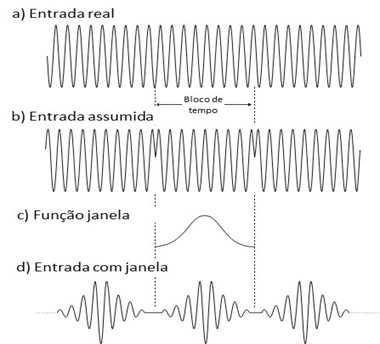
The FFT algorithm that transforms the input memory sample – digitized time waveform – into a spectrum, assumes that the data before and after the sample are similar. For this reason, the FFT algorithm needs the sample data to start and end at zero amplitude as seen in the figure.

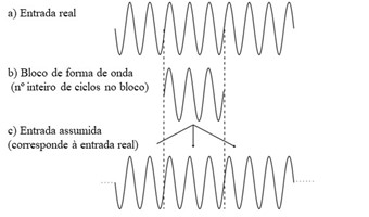
Note that the reconstructed waveform is the same as it was before sampling..

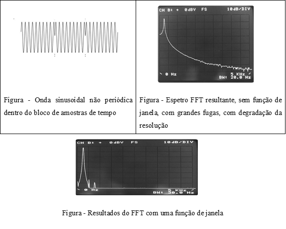
In the figure shown below, there was no sampling at zero amplitude, and a reconstructed waveform is obtained that is not the same as the original data. This waveform will cause errors in the spectrum called leaks. (leakage) - that is, the energy that exists in one line of the spectrum is dispersed by other adjacent ones.

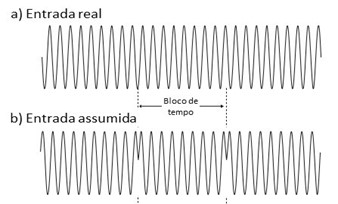
The resulting spectrum, shown in the following figure, implies loss of resolution.

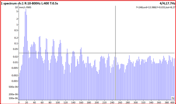
Note the spectral resolution around 1 Hz, on a spectrum in logarithmic vertical coordinates, of a vibration analyzer. Note that the energy in component a 17 Hz, corresponds to the speed of rotation, splits into several lines.

As data acquisition cannot be controlled to obtain periodic sampling, windows are used to force endpoints of data to zero, as shown in Figure.

Vibration data processing and theThe “Hanning” and “Uniform” windows

A window function is multiplied by each signal block to obtain a register that is zero at both ends.. Windows are not necessary and should not be used when the transient data obtained starts and ends at zero. A Hanning window destroys part of the data in a transient signal because important data at the beginning of a sampling can be eliminated as shown in Figure.

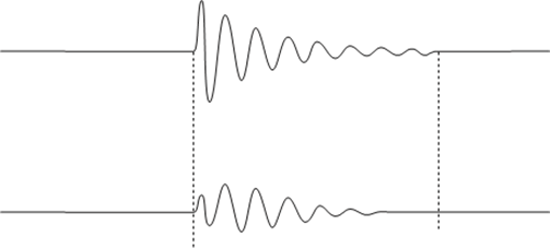
For transient data response can be used a “Uniform” window. The Hanning window has a limited filter inside the box or line that allows a good resolution bandwidth as seen in the figure..

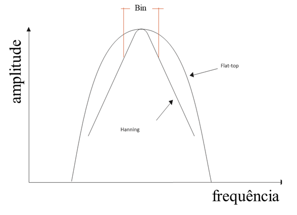
However, as it is limited inside the box, the inaccuracy of the amplitude (sometimes called bandwidth inaccuracy) can have the value of 1.5 dB (16%) if the measured frequency falls on the edge of the box as seen in the following figure.

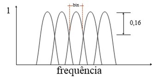
Flat-top window has lower resolution, but has only an amplitude inaccuracy of 0.1 dB (1%). Therefore, flat-top window is recommended for discrete spectral lines and amplitude accuracy. The Hanning window is recommended for stable data with multiple frequencies.. The current resolution for each window can be calculated using the window factor given in the Table below..

Table – FFT window selection

Window	Aim	amplitude uncertainty	window factor (WF)
Uniform	impact tests	56.5%	1
Hanning	breakdown analysis	16%	1.5
Flat top	Condition assessment	1%	3.8

Resolution = 2x line bandwidth = 2 x Fmax x (WF)/ number of lines

The analyzer's confidence resolution is twice the frequency range of the spectrum, multiplied by the window factor, divided by the number of rows selected.

Uniform or rectangular windows are used in impact tests, unless the data does not reach zero within the sample. For this reason, double taps within the data acquisition time, has to be avoided.

To learn more about this topic click here.

G vibration data processingloves Dynamics and “autorange”

Dynamic range refers to the ability of an analyzer to identify low amplitude components, in the presence of high amplitude components, not spectrum.

Dynamic range determines whether or not amplitudes at different frequencies can be determined.. Currently, most devices have 120 dB (24 bit) dynamic range. In the past, most data collectors, (16 bit) had 90 dB of dynamic range. for these equipment, one bit is used for the sign +/- (like this, 2¹⁵ = 32,768). This means that AC signals with a difference in amplitude up to 32,000 for 1 could be determined (DC signals from 64,000 for 1). Older 12-bit data collectors had a dynamic range of 66 dB (2048-1). In the past, if the input gamma of the FFT analyzer was set too high for the difference in amplitudes of the two signals, the dynamic range would not be enough to allow observing the lowest signal amplitude.

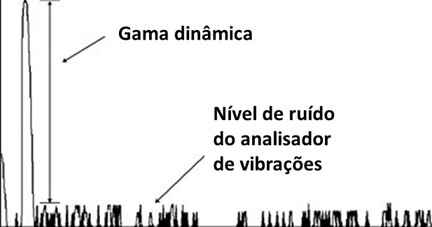
At the moment, com 120 dB of dynamic range, the equipment no longer needs any further scale adjustment.

Vibration data processing – Linear and logarithmic scales

In vibration analysis problems occur when acceleration or displacement are displayed in a spectrum, with a wide range of frequencies, and its components are shown at high and low frequencies. A wide dynamic range is obtained using a logarithmic amplitude scale, which are compressed scales.

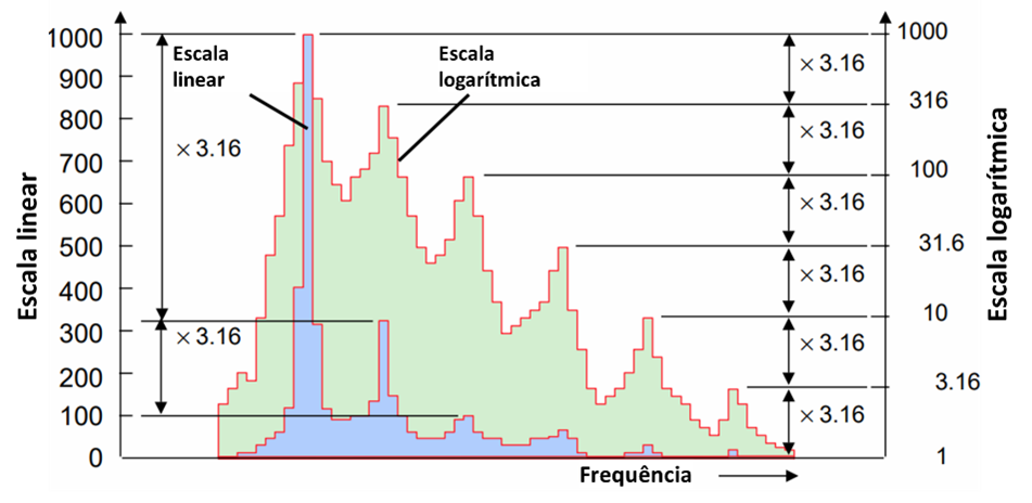
The previous figure shows both scales, linear and logarithmic. A second order that is just 0.1% (1/1000) the value of the first order, will not appear on the linear scale, more will appear less 60 dB than the first order on the logarithmic scale.

dB = 20 log V/V_ref, or dB = 20 log 1/1000 = -60

This situation can occur in the initial phase of bearing failure and the amplitudes are contained in a spectrum with significant amplitudes of vibration of the gears. An example is 17,4 mm/s the gearing frequency and 0,25 mm/s the frequency of bearing defects. The required dynamic range would be:

dB = 20 log 17,5/0,25 = 36,9 dB

This dynamic range is available on all modern data collectors.; Yet, dynamic range must be properly configured on the analyzer, or the autoscale function should be used (autorange).

It is important to have a good dynamic range when you want to measure low frequency accelerations or high frequency displacements in the presence of low frequencies..

The modern parsers, with analog to digital converters 24 bit and dynamic range 120 dB no longer need the autoranging function.

To learn more about this topic click here.

Vibration data processing and – as media

FFT analyzer can be used for average value calculation in addition to instant FFT display, after data is collected. These modes for calculating the average value, include rms, peak retention, synchronous time, and the overlap.

To learn more about this topic click here.

A media rms

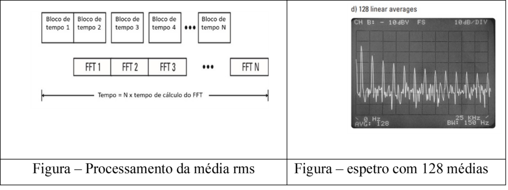
The average rms amplitude is obtained by averaging over the bins as each block of data is processed. Noise is smoothed, but not deleted, and discrete signals are reinforced on the screen.

The synchronous average in time

Synchronous averaging over time is performed on the waveform. One trigger is made available to the analyzer at the shaft frequency from a proximity sensor or an optical pickup.

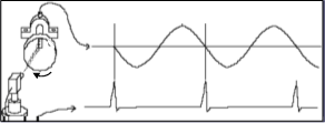
This technique consists of performing measurements of the waveform, synchronized with the rotation of one of the shafts and the execution of an average of these measures. As a result of this synchronization, asynchronous events with the realization of the average, tend to zero, while synchronous becomes more visible. Therefore, the periodic part of the entry will always be exactly the same in each block of time that we take, while the noise, it is clear, will vary. If we add a series of these blocks of time triggered by the tachometer and divide by the number of blocks we take, let's calculate what we call a synchronous mean in the time domain. With this technique we managed to eliminate from the waveform the vibrations that are not related to the shaft where the tachometer is located..

For example, The following figure shows the result of applying synchronous averaging over time to separate the vibration of two paper machine press rolls.

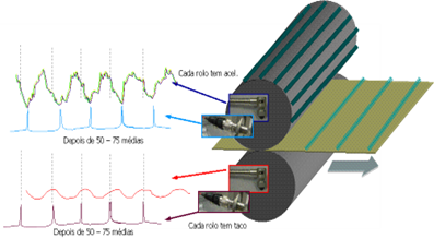
Synchronous time averaging eliminates non-synchronous noise in the signal.

The average peak retention

The peak hold function, retains the highest peak or rms value on each bin as each new block of data is processed. Therefore, Do not do, really, any average calculation. Peak hold function is used for transient tests. The major disadvantage of using FFT analyzers in transient testing is the long acquisition time required.. A block of data must be processed before it can be displayed.. Therefore, in a deceleration test, the machine may experience a wide change in RPM while a data sample is being collected. Each FFT Peak Hold associates only one point on the curve. It takes numerous points to describe the range around the critical speed..

Figure – Peak retention average is used to follow the amplitude of the largest peak of vibrations in the spectrum., during a machine stop and also to indicate speed variations over time

What is zoom and when is it used?

When you want to see in real time, a very noisy vibration, or vary, exponential average is used. Exponential average, time blocks do not contribute to the average equally. De facto, a new record weighs more than the old ones. The value at any point in the exponential mean is given by: Y [n] = and [n-1 * (1 – a) + x [n] * a onde:

• First of all, n is the umpteenth mean and the umpteenth new time block.
• Then, alpha is the weighting coefficient.
• Normally, alpha is defined as 1 / (Number of averages).

For example, on the analyzer, if the number of averages is set to 3 and the average type is selected as the exponential average, then α = 1/3. The advantage of this type of media is that it can be used without end. Unlike the average RMS, the exponential mean will not stop after n times. As mentioned, the RMS average ends after some number of averages. On the contrary, this type of average is kept running until we stop it. Thus, the average result changes as we acquire new records and will gradually ignore the effects of old records.

Negative mean

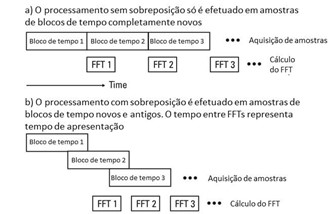
Processing overlay (overlap)

In overlapping processing, just a fraction of the new data, are collected in the input buffer. Previous sample data is used to make a complete sample for processing. The number of lines or bins, frequency range, and overlapping processing are considerations when the analyzer is set up for transient testing because they determine the acquisition time.

To learn more about this topic click here.

Vibration data processing – The envelope analysis

The envelope analysis is, currently, the tool par excellence, for detecting impacts such as those generated in bearing failures with a vibration analyzer. It has also become essential to diagnose all mechanical problems that can generate impacts, such as gears in poor condition, days off, desapertos, etc.

Originally, when it was developed did not have the ability to measure, with accuracy, the level of acceleration generated by mechanical impacts, but, since the nineties, with the development of detection technology impact peaks, this limitation is exceeded.

The envelope with vibration analysis techniques have had various commercial designations and, namely:

• PeakVue (Emerson/CSI);
• Espectro de Spike Energy (IRD/ENTEK/Rockwell Automation);
• demodulation;
• Envelope;
• Etc.

However despite the different names and how to implement, all continue to provide envelope analysis versions.

Envelope analysis – the frequency spectrum of waveforms generated by impacts

Often referred to the representation in the frequency spectrum of a sinusoidal vibration. When it comes to vibrations generated by impacts, of very short duration, vibration is not of the sinusoidal type and new challenges arise.

In the following figure you can see different types of waveforms and respective frequency spectra as measured by a vibration analyzer.

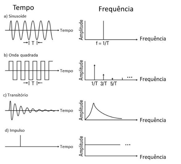
Figure - Waveforms and respective spectrum

The frequency spectrum of an impulse, similar to that generated by an impact, it's a flat line, low amplitude that spreads across all frequencies.

Envelope analysis – the measurement of vibrations generated by impacts

There are two technical challenges in measuring the vibrations generated by impacts:

• Separate the vibrations generated by impacts, What is the frequency spectrum of impact-generated waveforms like?, of other vibrations generated in a machine;
• Quantify, with accuracy, the level of vibrations generated by impacts.

Envelope analysis – separating the vibrations generated by very low level impacts

When it comes to measuring vibrations on a machine, we are often interested in detecting very low level impacts in the presence of other high amplitude vibrations on a machine.. This is the situation you face when trying to detect the first symptoms of a bearing failure..

If you manage to separate the vibrations of the impacts from the other existing vibrations in the machine, it will be much simpler to follow its growth, as shown in Figure.

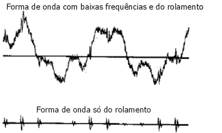
Figure The need to separate impact vibrations from other vibrations in machines

The figure below shows the vibrations generated by the small impacts of the first phase of bearing failures in the frequency spectrum..

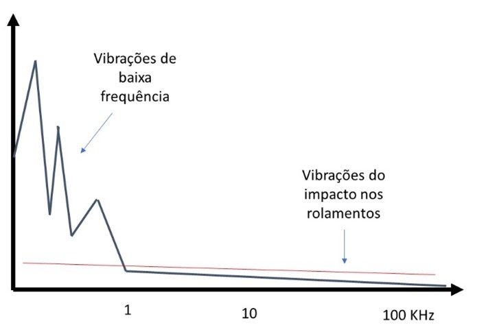
As the vibrations in the bearing degradation, in its early stages, arise especially in acceleration, at high frequencies, it is possible to separate / enhance the vibrations of the impacts, by using a high pass filter of the vibrations measures. In this way, it is possible to separate the vibrations of bearing impacts from the other vibrations of the machine..

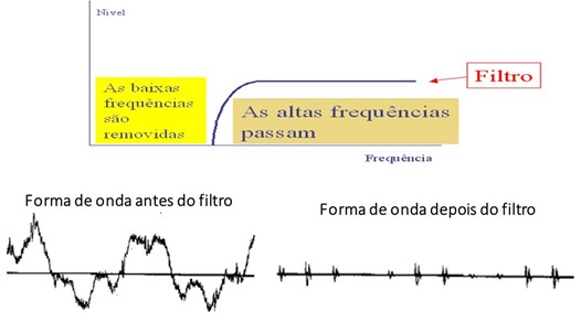
Figure Elimination of vibration at low frequencies – filter input high pass

This filtering operation is the first envelope with the vibration analysis.

Envelope analysis – quantifying the level of vibrations generated by impacts

The phenomenon of “aliasing” and the sampling rate necessary to measure, with accuracy, the level of a sinusoid in the frequency spectrum.

Imagine now that in order to see the characteristic frequencies of a bearing, you want to see a spectrum up to 1 KHz. As seen above, the waveform sample rate will be 2,56 times the Fmax of the spectrum ie 2,56 KHz. The time interval between each sample is 1/ 2560 seconds ie 0,4 mseg. If the duration of the impact is less than this time, the level of impact will not be adequately measured, as can be seen in the figure below.

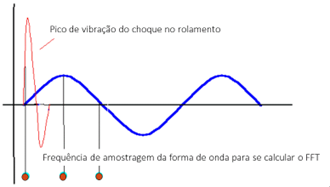
It has been so that the fixed relationship between sampling in time and frequency range, intrinsic mathematical function of Fourier transform, obtained with the FFT spectrum, prevents obtaining simultaneously:

• A high sampling enabling us to properly measure the levels of impact peaks;
• A high resolution in the frequency spectrum that allows to clearly identify the characteristic frequencies of faults in bearings.

The solution to this issue is to make the sampling rate independent of the waveform for detection of impact peaks from the sampling rate to obtain the FFT spectrum.. This is the solution that nowadays is implemented by some analyzer manufacturers.

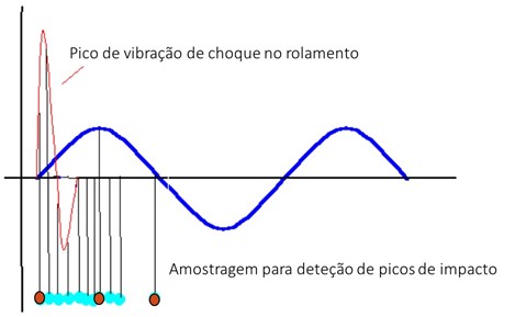
Figure Sampling rate of the appropriate waveform to characterize the vibration level generated by an impact

As shown in the figure, the sample rate, adequate to characterize the level of vibrations generated by impacts is much higher than that needed to characterize the level of a sinusoidal vibration.

The envelope analysis – the characterization of the repetition rate of impacts

To meet shock repetition period of the envelope analysis rectifies the waveform before performing the FFT spectrum.

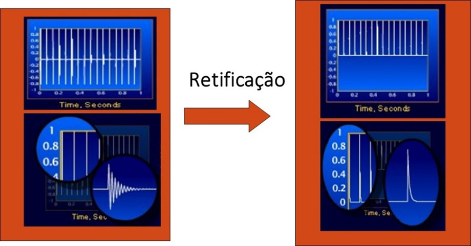
Envelope analysis – Obtaining the frequency spectrum of the traditional envelope

The frequency of vibration analysis is performed on the rectified waveform, There was thus having the following diagram of vibration analysis blocks with envelope.

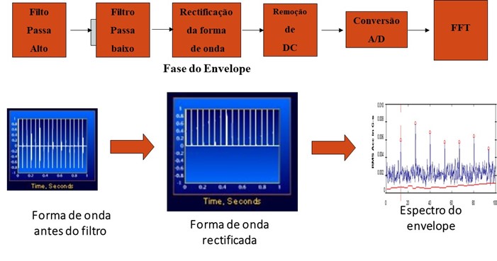
Figure - Scheme of implementation of vibration analysis with traditional envelope

This way of implementing the FFT spectrum does not adequately characterize the level of the components of the rectified waveform and the frequency spectrum.

The spectral map or cascade

Some FFT analyzers generate a waterfall diagram as shown in the following figure. This diagram contains a number of spectra taken at various speeds or times and, in some cases, space (that is, the analyzer stacks the spectra in a waterfall graph by measurement position).

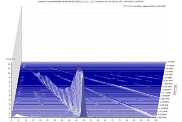
Figure Waterfall diagram or spectral map

Vibration data processing – The analysis by orders

When analyzing rotating machines, measured data will depend on rotation speed. Varying rotation speeds will change the characteristics of the measured data.

The components of the measured signal that change frequency with changes in speed, are referred to as rotational speed harmonics or orders.

The 1st harmonic component has a frequency equal to the rotational speed, indicated in Hz, and for example, the 10th harmonic has a frequency 10 times greater than the 1st harmonic. Velocity variations cause the relevant harmonic frequency components to change up and down in frequency..

If the machine is running at a perfectly constant rotational speed, then the harmonic orders in the FFT spectra would remain on the same spectral lines throughout the measurement. Actually, many machines will have some speed variations, even though they are set to run at a certain rpm value.

When using order analysis instead of FFT analysis, spectra will relate to vibrations per revolution rather than vibrations per second. Therefore, will be independent of the speed of rotation. This provides stable harmonic order patterns across varying speeds for rotation-related vibration components..

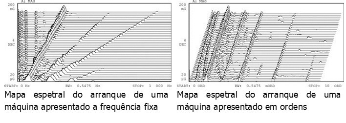
Another advantage of using order analysis for rotation-related measurements is to avoid widening the order-related spectrum components.. Stretching happens when the frequency pattern changes during the calculation of a spectrum. This can be either during the calculation of an instantaneous spectrum or across multiple instantaneous spectra that are measured together..

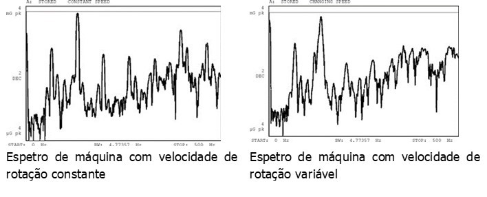
Broadened spectra will lack clear harmonic peaks, since the peak frequencies were changing during such spectrum calculations. Instead of clear harmonic peaks, the stretched spectra will spread the energy of the harmonic orders over the frequency ranges related to all the rotational speeds present during the spectrum calculation.

When using order analysis, spectral smearing is avoided for such non-stationary signals, since the harmonic components of rotation remain at fixed order positions in the order spectra.

In order to carry out the analysis by orders, information about the rotation speed of the machine is required., usually measured with a tachometer.

Vibration data processing – The graph of Bodé

The Bodé plot consists of the presentation of the amplitude of vibration (normally at 1xRPM) and phase versus spindle speed. This graph, can potentially provide a lot of information not available from steady-state measurements like the FFT. The most common use of Bodé is to identify the natural frequencies present in machines. The most common are the calls “critical speeds” that occur when the rotational speed of the shaft coincides with a natural frequency and produces a resonance. This appears as an amplitude peak and phase shift on the Bodé plot..

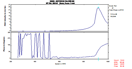
Identification of natural frequencies is especially critical in turbomachinery because, unlike most general purpose equipment, work above or near a, if not more, natural frequencies or modes. The Bodé plot is more powerful in identifying synchronous vibrations. While the overall vibration can also be plotted against the shaft speed, the Bodé plot is not really a tool to identify non-synchronous vibrations.

Vibration data processing – why is it important when looking at speed variation in a machine (Nyquist)

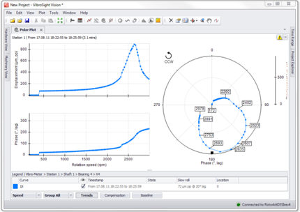
The Polar chart displays exactly the same data as the Bodé chart, just in a different display format. in the polar portion, the magnitude of the displacement vector is measured radially, from the center of the graph and the phase is plotted circumferentially. A resonance is indicated on a graph by the speed at which the amplitude is the maximum of a circle. (that is, approximately 180 degrees of phase change).

Vibration data processing – Measuring the Frequency Response Function

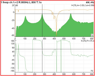
This function is used to determine the natural frequencies of a structure from an impact test..

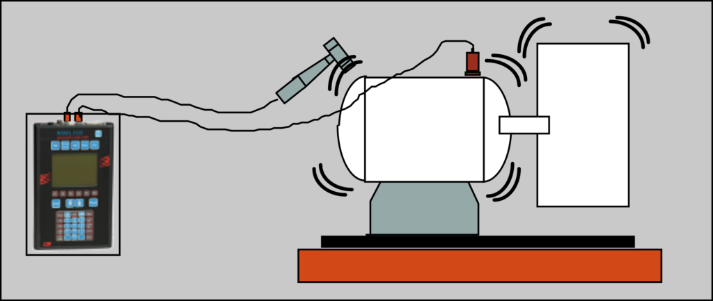
This essay is based on the principle that any structure when free, vibrates at its natural frequencies. Therefore, to observe its natural frequencies just, for example, make an impact on the structure and observe the vibratory response.

There are two ways to look at the impact.

• The simplest way is to measure only the response; the so-called impact test.
• The most elaborate way is to measure the Frequency Response Function (FRF). This is obtained using a hammer instrumented with a force transducer in order to know the energy that is being introduced into the structure.. This way of measuring the natural frequencies is more accurate and allows the comparison of the measured results with finite element models and modal analysis..

Measuring the frequency response (FRF) in addition to one of the functions described above, it provides information about the phase of the vibrations and the coherence function.

In a measurement of the Frequency Response Function the following can be observed:

• resonances – The peaks indicate the presence of the natural frequencies of the structure under test;
• Damping – Damping is proportional to the width of the peaks.. The wider the peak, the greater the damping;
• vibration mode – The amplitude and phase of multiple acquired FRFs relative to a common frame reference are used to determine the mode shape..

Coherence is function versus frequency, which indicates how much of the output is due to the input in the FRF. May be an indicator of FRF quality. Evaluates the consistency of the FRF from measurement to repeating the same measurement. The value of a coherence function varies between 0 e 1.

in a vibration analyzer as part of a program of, unequivocally defines that we are in the presence of a natural frequency because, in resonance the phase varies 180º. If this variation is less than 180º, it means that, or the structure is heavily cushioned or else, that the movement of the structure in the resonance does not occur in the direction of the accelerometer and / or the hammer.

Vibration data processing, cFFT Analyzer and Data Collector Configuration

The purpose of the FFT analyzer setup is to produce data upon which decisions can be made regarding faults and operating condition.. Machine knowledge is essential; that is, breakdown frequencies, natural frequencies, and amplitudes of critical failures. It is well known that all these data will not be available when a machine is monitored or analyzed for the first time.. Yet, as time passes and the analyst works with a machine, experience gained will provide information about the vibration levels at which defects appear that lead to failure. Frequency information relating to faults such as spindle speed, bearing frequencies, passing frequencies of blades or blades, and gearing frequencies should be available at the start of monitoring or analysis. IS, therefore, possible to make a reasonable configuration based only on the project data. The two main issues that must be considered are resolution (frequencies) and dynamic range (amplitudes).

Vibration data processing and resolution of the spectrum

Spectrum resolution is dependent on the number of lines used in the FF calculation (which is related to the number of waveform samples in the input buffer, the frequency range, and the chosen window. The minimum resolvable frequency is the inverse of the data acquisition time. In other words, must be present in the data block, a complete block (a period) of data to the frequency in question, before this frequency is observed in the spectrum.

For example, it is intended to analyze data at a frequency of an operating speed of 1800 RPM (30 Hz), then [1/30 = 0.033 s/cycle]. A minimum of 33 ms of data, must be collected. Otherwise, the vibration to 30 Hz did not cycle during the data acquisition process.

Frequencies cannot be separated between lines. This fact is important in relating frequency range and number of rows to the lowest resolvable frequency.. If they are chosen 400 lines, the spectrum will be divided into 400 discrete points, with all frequencies falling between the charged lines on its adjacent line. The analyzer shows the frequency in the center of the bin. For example, if a frequency range of 1000 HZ had been chosen in the example, lowest resolvable frequency would be 1000Hz/400 lines, or 2,5 Hz. So it should have been picked up, 400 ms (1/2,5 = 0,40 second) of data, e 30 Hz could be determined.

Vibration data processing – Bugs and noise due to windows

Errors and noise are introduced when windows are used in FFT processing. For this reason a window factor (noise factor) is used to calculate the guaranteed resolution. The theoretical resolution of the frequency range divided by the number of lines must therefore be decreased by multiplying the window factor twice..

When a data logger is used to conduct fault diagnosis or condition assessment, a waveform must be saved with each spectrum. If data is being recorded, the data stored must be sufficient so that the FFT analysis can be conducted for the desired frequency ranges and resolution.