Vibration analyzer 6 – Ace Media
Then, on vibration analyzer 6, we present the theme of averages, a vibration analyzer. Like this, this article is part of a series of articles that explain how a vibration analyzer works.
When we do Vibration Analysis, we need to understand how an analyzer works. Therefore, here we present the concepts of digital signal analysis, implemented in an FFT analyzer. In order to be easy to understand, we always present them from the user's point of view, in a vibration analyzer when performing predictive maintenance.
Then, no link, we can see a range of Vibration analyzers provided by D4VIB.
Then, in Vibration Analyzer 6, we present the content of this series of articles.
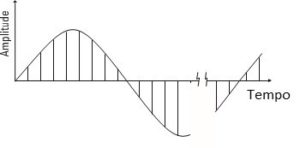
- What is the relationship between time and frequency
- How sampling and scanning works
- What Aliasing is and what effects it has
- How it is used and what the zoom consists of
- How waveform windows are used
- What are averages for
- What is real-time bandwidth
- What overlay processing is for (“overlap”)
- What is order tracking
- What is envelope analysis
- The two-channel functions in the frequency domain
- What Orbit is for
- What are the functions of a channel in the time domain
- What the Cepstro consists of
- What are the units and scales of the spectrum
6 – Vibration analyzer 6 – What are averages and what are they for in an analyzer
In such a way that the operation of an analyzer, be easier to understand, we often use examples of noise-free signals. However, as how they are carried out as. actually, we often measure the actual vibration, in the presence of a significant noise level. On the other hand, on other occasions, the vibrations you are trying to measure, are very similar to noise.
Like this, due to these two common conditions, we have to develop techniques for:
- First of all, measure signals in the presence of noise,
- Then, measure the noise itself.
actually, we know from statistics that the most common technique for improving the estimation of a value to vary, consists of averaging.
Similarly, when we see a noise reading on an analyzer, we can try to guess the average value. On the other hand, how analyzers have the ability to perform calculations, we can ask them to calculate the average value.
6.1 – What is the average RMS
It should be noted that, when we look at the spectrum and try to estimate the average value of the spectrum components, we are in fact doing a simplified average of the level. De facto, we are trying to determine, “the eye”, the average of the signal.
De facto, this technique of averaging, is very valuable in determining the average level, on any of the spectrum lines. The more averages we make, the better the average level estimate will be.
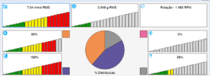
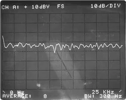
For example, in the figure 6.1, we see average spectra of:
- Random noise from a function generator,
- Signal originating from a function generator,
- Human voices measured with a microphone.
De facto, in these signs, the instantaneous value of each component of the spectrum varies widely. On the other hand, when we see the average value, we can see the basic properties of the spectra well.
a) Here you see the random noise spectrum
c) Here we see the spectra corresponding to people's voices
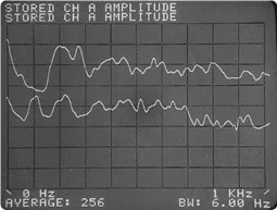
- The upper graph shows: female voice
- The bottom graph shows: male voice.
Figure 6.1. In these figures we see the result of using the RMS average.
De facto, RMS means “middle-quadratic root”, and is calculated as follows:
- First of all, the sum of squares of individual values is calculated, divide by the number of measurements.
- Then, is the square root of the sum.
actually, if you want to measure a small signal in the presence of noise, the average RMS gives a good estimate of the signal plus noise.
On the other hand, with the average RMS, you cannot improve the signal-to-noise ratio.
De facto, with this kind of average, we only make more accurate estimates of the result of the sum of the signal plus the noise.
6.2 – How it works and what is the average time (or synchronous)
6.2.1 Firstly, what does this average consist of
Sometimes, in order to improve the signal-to-noise ratio of a measurement, we use linear mean in the time domain. We can use this technique, when we have a tachometer signal.
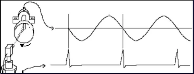
Figure 6.2 – In this figure, we see the use of the tachometer, for synchronized measurement with machine rotation.
Like this, when using this technique, the tachometer is used to trigger the start of a time block record.
In this conditions, the periodic part of the entry will always be exactly the same, in every block of time that we take. De facto, the more averages we do the more the result will tend to the waveform, which is repeated in all blocks of time.
On the contrary, since the noise is different in each block of time, will tend, with the average, to go to zero. De facto, the more averages we take, closer the noise reaches zero.
Thus, the signal-to-noise ratio of our measurement is improved.
6.2.2 Examples of applying time averaging
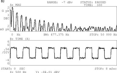
For example, figure to follow, shows a time block of a square wave, hidden in noise. De facto, after 300 media, the average of the resulting time block, the signal / noise ratio has a marked improvement. actually, the square wave is seen in a much better way.
Thus, when calculating the FFT of the average time block, we see many more harmonics. actually, as harmónicas, because of the reduced noise level, can be accurately measured.
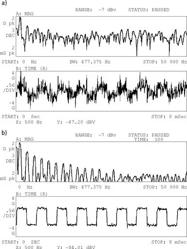 a) First of all, you see the spectrum and the waveform, resulting from a single block of time.
b) Then, you see the spectrum and the waveform, resulting from 300 time block averages.
Figure 6.3. Here we see the result of applying 300 media, in a square wave with noise.
6.3 What is the average peak retention for (peak hold)
Next, let's look at the topic of average peak retention. De facto, this average is different from the previous ones. Like this, this technique works by displaying and retaining the maximum level, at each frequency, over a succession of measures. Like this, can provide a history of maximum levels, every frequency, along the measurements made.
Then, in the figure, we present two application examples.
First of all, in (a), peak retention was used during a machine stop. Like this, this graph shows the maximum level at each frequency. Normally, this maximum level occurs at 1 x rpm.
In this case, the bottom graph (b), is a peak retention over a relatively long period. During this period the speed variation of a variable speed motor occurred. Like this, this chart can be used, for example, as an indication of load variation.
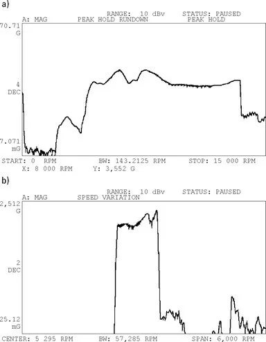
Figure 6.4 Peak hold average is used to track peak vibrations when a machine is stopped and indicate speed variations over time.
6.4 The Exponential Average
To complete, when you want to see it in real time, a very noisy vibration, or vary, exponential average is used.
Exponential average, time blocks do not contribute to the average equally. De facto, a new record weighs more than the old ones.
The value at any point in the exponential mean is given by:
Y [n] = and [n-1 * (1 – a) + x [n] * a
at where:
- First of all, n is the umpteenth mean and the umpteenth new time block.
- Then, alpha is the weighting coefficient.
- Normally, alpha is defined as 1 / (Number of averages).
For example, on the analyzer, if the number of averages is set to 3 and the average type is selected as the exponential average, then α = 1/3.
The advantage of this type of media is that it can be used without end. Unlike the average RMS, the exponential mean will not stop after n times.
As mentioned, the RMS average ends after some number of averages. On the contrary, this type of average is kept running until we stop it. Thus, the average result changes as we acquire new records and will gradually ignore the effects of old records.