Vibration analyzer 1 – The relationship between time and frequency
Then, on vibration analyzer 1, we review the relationship between time and frequency, in a vibration analyzer when performing measuring vibrations. Like this, this article is part of a series of articles that explain how a vibration analyzer works.
actually, when we carry out the Vibration Analysis, we need to understand how an analyzer works. Therefore, here we present the concepts of digital signal analysis, implemented in an FFT analyzer. In order to be easy to understand, are always presented from the user's point of view, in a vibration analyzer when performing predictive maintenancea.
Then, no link, we can see a range ofVibration analyzers provided by D4VIB.
Then, on vibration analyzer 1, we see the content of this series of articles.
- What is the relationship between time and frequency
- How sampling and scanning works
- What Aliasing is and what effects it has
- How it is used and what the zoom consists of
- How waveform windows are used
- What are averages for
- What is real-time bandwidth
- What overlay processing is for (“overlap”)
- What is order tracking
- What is envelope analysis
- The two-channel functions in the frequency domain
- What Orbit is for
- What are the functions of a channel in the time domain
- What the Cepstro consists of
- What are the units and scales of the spectrum
1 – Vibration analyzer 1 – The relationship between time and frequency
1.1- How FTT works and moves from time to frequency
First of all you have to take into account that with the Fast Fourier Transform ( Fast Fourier Transform – FFT) past time domain data, for the frequency domain. Like this, this even seems easy to implement because that’s what we want an analyzer to do. However, we will see that there are many factors that complicate this task.
On the other hand, to dispose of the results expeditiously, we have to calculate the FFT automatically. However, we can only calculate the FFT, after sampling and digitizing the input waveform.
Therefore, this calculation cannot be performed continuously. Like this, this means that, the algorithm transforms complete blocks of data into the time domain, in frequency spectra.
Then we see:
- a) The waveform in volts
- b) The sampled waveform
- c) The frequency spectrum

Figure 1.1 – The time block samples, in the time domain, and the lines in the FFT spectrum in the frequency domain
As referred, in none of the domains there is an exact representation . However, we get a representation of the sampled waveform. De facto, this presentation is very close to the intended.
Then, what is the sample spacing in the time block?, to ensure the desired resolution, in frequency.
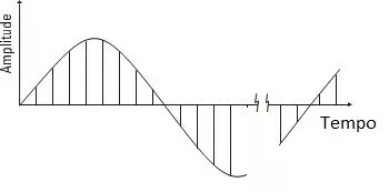
Figure 1.2 A time block is made up of N equally spaced samples, of the analog waveform of the vibration sensor signal, that enters the vibration analyzer.
1.2 – Vibration analyzer 1 – How the waveform samples form the time block
In other words, a block of time is defined as being made up of:
- An N number, of waveform samples,
- Since these samples are consecutive,
- And that these samples are evenly spaced.
There is also a need to, to make the calculation simpler and faster, the number N is always a power of 2. Like this, it is because of this that, analyzers it is common to find line number options such as 512, 1024, 2048, 4096, etc. De facto, these numbers are all powers of 2.
There is also a need to, the time block is transformed as a everything, on one block full of frequency lines, that is, on a spectrum. Like this, it is therefore worth noting that, to calculate each line in the frequency domain, all samples of the time block are required.
Therefore, it is crucial to assimilate that the FFT, has the property to perform block calculations.
This is effectively necessary, to understand many of the features of an Analyzer.

Figure 1.3 The FFT is calculated on blocks of waveform samples.
1.2.1 As the block of time is transformed into a spectrum
In other words, the FFT cannot be calculated, until a complete block of time has been acquired.
In other words, this is so, why, as already mentioned, the FFT transforms the time block, as a whole.
However, once the calculation is complete, the oldest sample of the time block can be discarded. Therefore, when a new sample is added to the beginning of the time block, all samples are moved in the time register and form a new block. Like this, following the acquisition of the first block, we have a new time block, each time a new sample is acquired in the time domain. Thus, every time there is a new sample in the time domain, we can have a new spectrum.

Figure 1.4 A new block of waveform samples is obtained after each new waveform sample is acquired
Therefore, until we acquire a complete time block, we don't have a valid spectrum. After this, in the on-screen spectrum of the vibration analyzer there are rapid changes.
It should be noted that the presentation of a new spectrum, for each new sample in the time block, is generally information to vary with excessive speed. In fact this, oftentimes, would result in the presentation of thousands of spectra per second.
De facto, forward, in the sections on width of real time band (7) e overlap processing (8), there are the various implications of the speed with which a vibration analyzer calculates the FFT.
1.3 – The number of lines in the frequency spectrum
It has been previously mentioned that, the time block consists of N equally spaced samples.
Like this, another FFT property, is that it transforms these N samples into the time domain, in N / 2 lines, evenly spaced, I don't expect.
De facto, you only get half the lines, because each frequency line, contains two pieces of information:
- A amplitude
- A fase
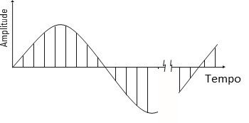
As it is known, the basic principle of FFT, is that the waveform can decompose into a sum of a series of sines of varying amplitude and frequency.
De facto, this is seen more easily if we look at the relationship between the time and frequency domains.

Figure 1.5 The relationship between the time and frequency domains.
Effectively so far, it is implied that, to reconstruct to waveform, the amplitude and frequency of the sine waves contain all the necessary information. Undoubtedly, it is obvious that the phase of each of these waves, it is also important. For example, in the figure 1.6, when thephaseof the highest frequency sine wave (the bottom), is changed, this results in a major change in the original waveform.

Figure 1.6 The phase of frequency domain components is important.
1.4 – How long the block of time lasts
Next we will see that, the lowest frequency that can be seen with the analyzer, is based on the duration of the time block.
actually, if the period of the input signal is greater than the duration of the time block, you cannot determine its period. In other words, lower frequencies cannot be determined. Therefore, the first line of the spectrum has an equal frequency, reciprocal of the duration of the block of time.
a) Input signal period equals time block. Lowest observable frequency.

b) On the contrary in this figure, the longest input signal period, is longer than the time block. Therefore, the FFT cannot calculate, the lowest frequencies of the input signal.
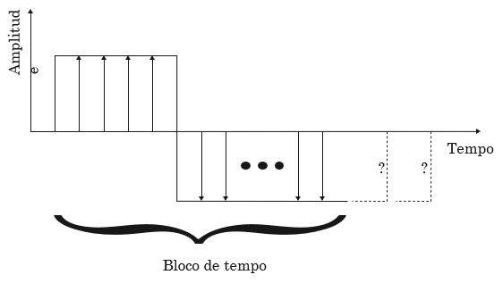
Figure 1.7. O, the inverse of the time block duration is the lowest observable frequency in the spectrum.
In addition, it must also be borne in mind that zero Hertz (DC), there is a frequency line. In fact, this line represents the average waveform input.
It is effectively known that, in vibration analysis this line is rarely used. De facto, to use, we need an accelerometer that measures the component at zero Hz. Effectively, it is to be noted that, the piezoelectric accelerometers, normally used, do not have this ability.
1.5 – Line spacing in the frequency spectrum
Therefore, in the frequency spectrum, the spacing between two consecutive lines is the reciprocal of the duration of the block of time.
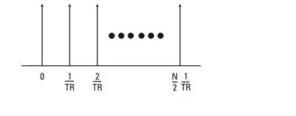
Figure 1.8 – Frequency spacing of all spectrum lines
1.6 For what reason, when looking at high resolution spectra, an analyzer is slower
Below we will mention what will happen, when we ask the analyzer to present a high resolution spectrum.
It should be noted that, due to the fact that the resolution is high, the value of the frequency range corresponds to a relatively small number. Like this, the duration of the block of time that is acquired to calculate the spectrum, which is its reverse, it's relatively large.
That way, in order to present the first spectrum, the analyzer will take a relatively long time. De facto, this is because you will acquire a long-term block of time.
In other words, it is faster to acquire low resolution spectra than high resolution spectra.
actually, you have to take into account that the calculation speed of the analyzer has nothing to do with this characteristic.
De facto, this characteristic is intrinsic to the FFT calculation formula.
1.7 – What is the maximum frequency of the spectrum?
We have already seen that in a spectrum there are N / 2 lines, spaced apart. We also know that, the value of this spacing is equal to the reciprocal of the time block duration. So you have to, to determine the highest frequency that we can see in a spectrum, this formula is used:

Therefore, we have that the frequency range of the vibration analyzer is determined by the sampling rate of the time block.
In other words, when an analyzer is asked to calculate a spectrum with a given maximum , with a certain number of lines, it is being defined simultaneously:
- The desired resolution in frequency.
- The duration of the time block.
It is effectively known that , the number of lines in the spectrum also implies a certain number of samples in the time block. To do this, over the duration of the block, the analyzer varies the sample rate so that it has N samples.
Thus, to reach the highest frequencies, the sample analyzer more quickly.
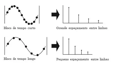
Figure 1.9 – The frequency range of vibration analyzers is determined by the sampling rate of the time block.
If you want to see a presentation of the topic covered in Vibration Analyzer 1, click here.