Vibration analyzer 13 – Functions of a channel in time
Vibration analyzer 13
The specific topic dealt with in a vibration analyzer 13, consists of the functions of a channel in the time domain in a vibration analyzer.
When it takes placeVibration Analysis, in a vibration analyzer when performing predictive maintenance, to take advantage of the full potential of a vibration analyzer, you need to understand how it works. Therefore, here are presented the concepts of digital signal analysis, currently implemented on an FFT vibration analyzer, from the user's point of view.
We begin by presenting the properties of the Fast Fourier Transform (FFT) on which Vibration Analyzers are based. Then, it shows how these FFT properties can cause some undesirable characteristics in the analysis of the spectrum, like aliasing and breakouts (leakage). Having presented a potential difficulty with the FFT, shows what solutions are used to make vibration analyzers practical tools. The development of this basic knowledge of the characteristics of the FFT makes it simple to obtain good results with a vibration analyzer on a wide range of measurement problems.
Here you can see the range ofVibration analyzers made available by D4VIB.
- What is the relationship between time and frequency
- How sampling and scanning works
- What Aliasing is and what effects it has
- How it is used and what the zoom consists of
- How waveform windows are used
- What are averages for
- What is real-time bandwidth
- What overlay processing is for (“overlap”)
- What is order tracking
- What is envelope analysis
- The two-channel functions in the frequency domain
- What Orbit is for
- What are the functions of a channel in the time domain
- What the Cepstro consists of
- What are the units and scales of the spectrum
13 - Vibration analyzer 13 - Functions of a channel in the domain in time
13.1 Vibration Analyzer - Basic measurement of waveform amplitude
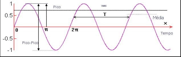
The vibration amplitude, which is the characteristic that describes its severity, It can be measured in several ways. In the following figure, one can see the relationship between the peak-peak amplitude, or Pico, Media and the Effective Level (RMS).
 Vibration analyzer 13 - Figure 13.1 Vibration analyzer - The RMS level, the peak and the peak-peak
The peak-peak value is important in indicating the maximum vibration amplitude, which is an important parameter when it comes to knowing for example, maximum displacements in machine tools or in measurements made with displacement transducers.
The Effective Value (RMS) it is the most frequently used because it takes into account a certain measurement time interval and gives a value that is directly related to the energy of the vibration, that is, its destructive capacity; is, therefore, an average value.
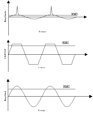
In the following figure one can see displayed three waveforms with the same peak amplitude and with different effective values. In a piggyback pulse comes to a sine, another is a sine, another is a truncated sine.
 Vibration analyzer 13 - Figure 13.2 - Vibration analyzer - Three waveforms with the same peak amplitude and with different effective values
The pulses that can be observed in the first waveform, of the previous figure, if they occurred in a rotary machine correspond to shocks. Peak amplitude measurement better detects shocks or any other type of impulsive phenomenon, measuring the RMS amplitude, due to the latter being an average value in a given interval while the peak value is, by definition, the maximum signal in time. To measure vibrations without effective pulse amplitude (RMS) It is due most suitable to provide an average value. To measure sinusoidal vibrations, whatever, because there is a fixed relationship between the peak amplitude and the RMS.
13.2 The Crest Factor
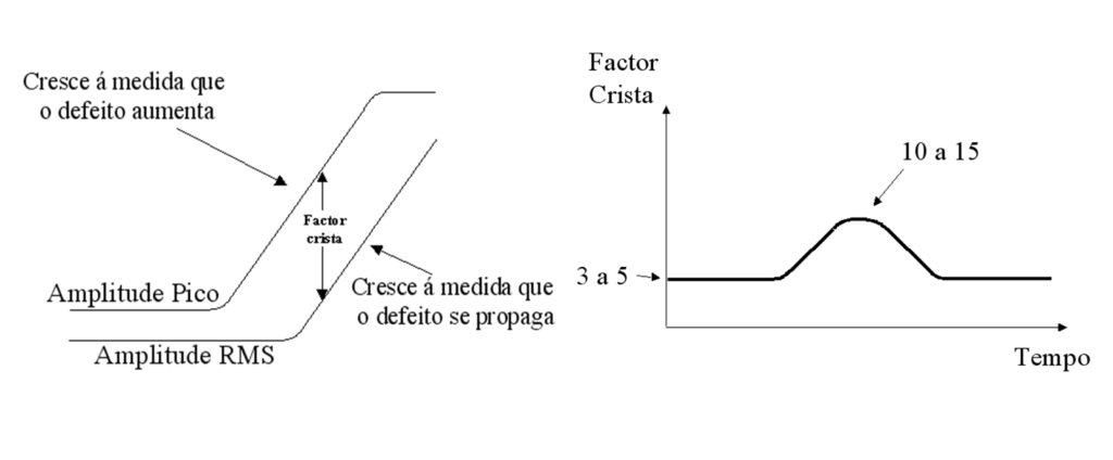
The Crest Factor is the result of the division between the Peak Value and the RMS Value of the vibration and is a technique to characterize the “impulsivity” existing in a waveform.
 Vibration analyzer 13 - Figure 13.3 - Vibration analyzer - The crest factor
The curves in the figure above shows a typical evolution of Crest Factor as the operating condition of the bearing deteriorates. Initially, there is a relatively constant ratio between the peak value and the RMS value. The peak value will grow normally until a certain limit. As the bearing deteriorates, more pulses will be generated for each passage of the balls, ultimately influencing the RMS values, even though the individual amplitude of each peak is not greater. By the end of bearing life, Crest Factor may have gone down to its original value, even, However, peak and RMS values have grown considerably. The best way to present the results of the measures is presented; the Peak and RMS values on the same graph, Crest factor with the deduced from the difference between the two curves.
13.3 O Kurtosis
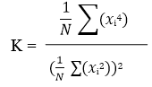
Kurtosis is a statistical indicator of the occurrence of large peaks in a waveform (impulsivity). No real world, many types of vibration are characterized by signals with a high Kurtosis value (in relation to the Gaussian random signal). The potential for fatigue and damage from these vibrations is greater than a pure Gaussian replication. Kurtosis can be expressed as a normalized “K” value by dividing the fourth statistical moment divided by the square of the second statistical moment. The equation below shows the Kurtosis calculation for N samples.

Vibration analyzer 13 - Figure 13.4 - Vibration analyzer - Waveform, peak value and Kurtosis
13.4 Asymmetries in the amplitude of the waveform
Observe the symmetry of the waveform data, above and below the axis of the center line, is important. Symmetrical data indicates that the movement of the machine is uniform on each side of the central position. Non-symmetrical data from the time waveform indicates that movement is possibly restricted by misalignment, friction or other external force.
 Vibration analyzer 13 - Figure 13.5 - Vibration analyzer - Asymmetric waveform generated by impacts on a bearing
13.5 The synchronous mean of the waveform
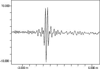
As was mentioned in detail in 6.3, this technique consists of making measurements of the waveform, synchronized with the rotation of one of the shafts and the execution of an average of these measures. As a result of this synchronization, asynchronous events with the realization of the average, tend to zero, while synchronous becomes more visible. Therefore, the periodic part of the entry will always be exactly the same in each block of time that we take, while the noise, it is clear, will vary. If we add a series of these blocks of time triggered by the tachometer and divide by the number of blocks we take, let's calculate what we call a linear mean in the time domain. With this technique we are able to eliminate vibrations that are not related to the shaft in the form of waves in which the tachometer is located, as for example you can see below , in the figure 13.6 to identify a gap in a gear.
Vibration analyzer 13 - Figure 13.6 - Vibration analyzer - Detection of cracks in gears through the Synchronous Average of the Waveform
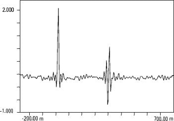
For the implementation of this technique, the existence of a tachometric sensor is required that permanently informs the measuring equipment about the rotation speed of the shaft where the measurements are being carried out. how they are carried out. This technique has traditionally been applied to complex and highly responsible gears such as helicopters for determining tooth defects., and in presses of paper machines or rolling mills to determine the source of vibrations in order to avoid quality problems. It allows, for example, on two rolls of a press rotating at the same speed, distinguish the vibrations generated by a, of the vibrations generated by the other, as illustrated in Figure 13.7
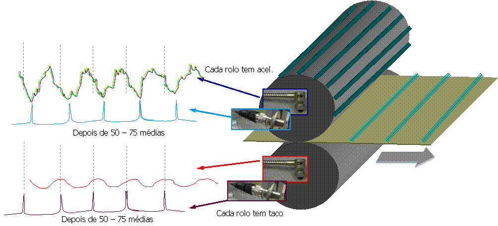 Vibration analyzer 13 - Figure 13.7 - Implementation of synchronous average in paper machine press rolls
The synchronization of measurements acts as a filter that allows us to exclusively observe / separate the vibrations from one source from the others..
13.6 Vibration analyzer 13 - Autocorrelation
Self-correlation is a correlation technique that involves only one signal, and provides information about the periodicity of the signal in the domain in time. Self-correlation, appears like this, as an alternative to spectral analysis. The main features of this function are:
• the ability to identify low repetition events,
• the ability to identify and separate periodic events from random events.

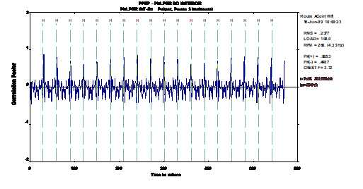
Vibration analyzer 13 - Figure 13.8 - Vibration analyzer - Application of the auto-correlation function to identify the absence of periodicity, that is, the random character of a vibration signal when a lubrication problem occurs in a bearing
A vibration analyzer usually has the ability to display the time stamp on your screen. This is the same waveform that we would see with an oscilloscope, a time domain view of the entry. But there are other time domain measurements that a Vibration Analyzer can also take. These are called correlation measures. Let's start this section by defining the correlation and, then, we will show you how to make these measurements with a Vibration Analyzer.
Correlation is a measure of the similarity between two quantities. To understand the correlation between two waveforms, start by multiplying these waveforms in each instant and adding up all the products. He, as in Figure 13.9, the waveforms are identical, each product is positive and the resulting sum is large.
 Vibration analyzer 13 - Figure 13.9 - Vibration analyzer - Correlation of two identical vibrations
He, However, as in Figure 13.10, the two records are different, so some of the products would be positive and some would be negative. There would be a tendency for products to cancel, so the final sum would be less.
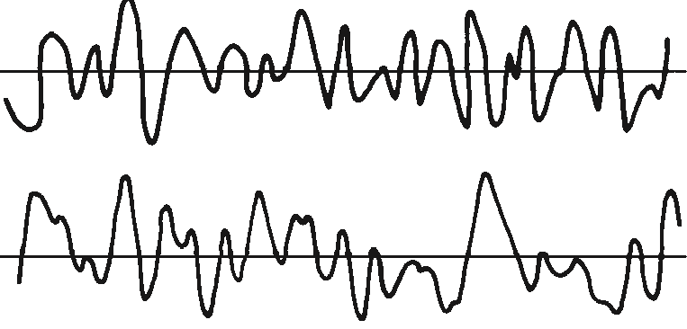
Vibration analyzer 13 - Figure 13.10 - Vibration analyzer - Correlation of two different vibrations
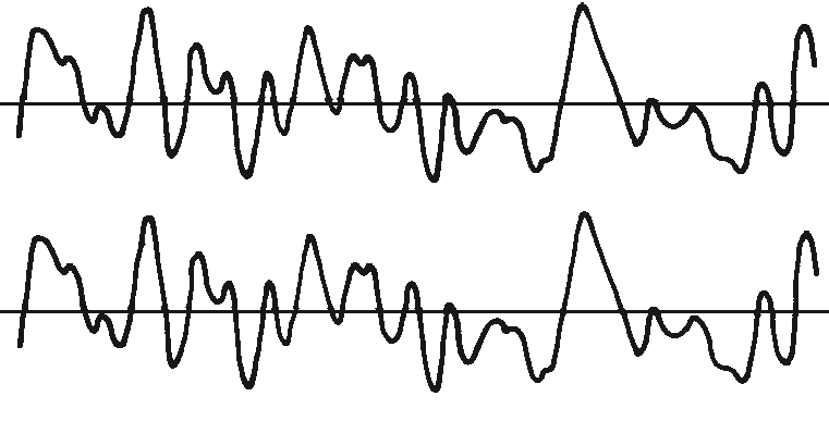
Now consider the waveform in Figure 13.11a and the same waveform that was delayed in time, Figure 13.11b. If the time delay was zero, then we would have the same conditions as before, that is, the waveforms would be in phase and the final sum of the products would be large. If the time change between the two waveforms is large, However, the waveforms look different and the final sum is small.
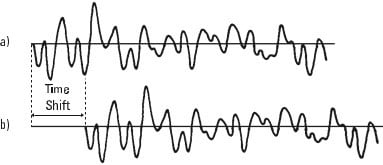
Vibration analyzer 13 - Figure 13.11 - Correlation of two identical vibrations, but lagged in time
Going one step further, we can find the average product for each time delay, dividing each final sum by the number of products that contribute to the same. If we now see the graph of the average product as a function of the time delay, the resulting curve will be greater when the time delay is zero and will decrease to zero as the time delay increases. This curve is called the automatic waveform correlation function. It is a graph of the similarity (or correlation) between a waveform and itself, depending on the time change.
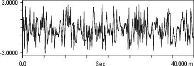
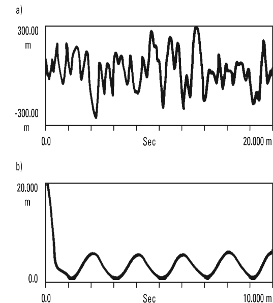
The auto-correlation function is easier to understand if we look at some examples. The random noise shown in Figure 13.12 is not similar to itself with any amount of time delay (that's why it's random) so your auto-correlation has only a peak at the point of 0 time delay.
a) Random noise temporal recording
b) Automatic random noise correlation
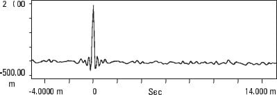
Vibration analyzer 13 - Figure 13.12 - Vibration analyzer - Random noise correlation
The pseudo-random noise ( stretches of random noise periodically repeated), However, repeats periodically, so when the time delay is equal to a multiple of the period, auto-correlation is repeated exactly as in Figure 13.13.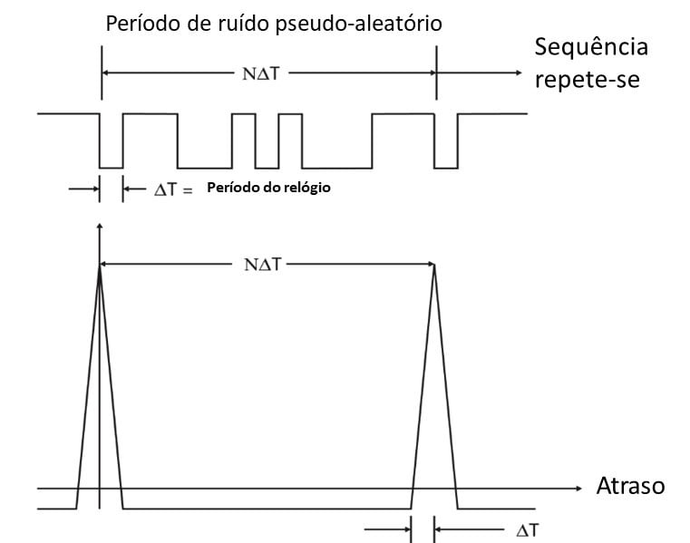 Vibration analyzer 13 - Figure 13.13 - Vibration analyzer - Pseudo-random noise correlation
These are both special cases of a more general statement; the auto-correlation of any periodic waveform is periodic and has the same period as the waveform itself.
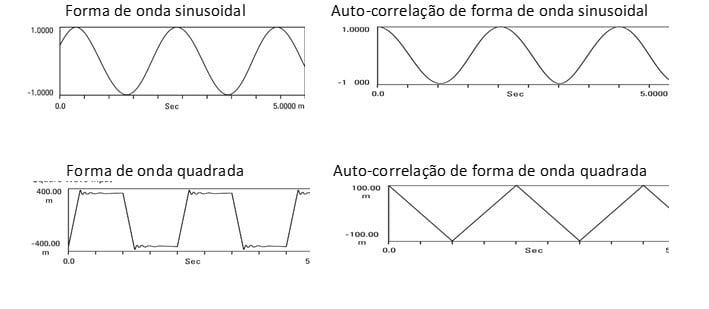 Vibration analyzer 13 - Figure 13.14 - Vibration analyzer - Periodic wave auto-correlation
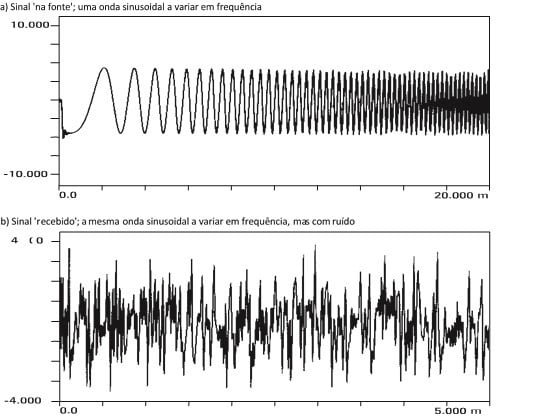
This can be useful when trying to extract a signal hidden by noise. Figure 13.15a shows what appears to be random noise, but actually there is a low level sine wave buried in it. We can see this in Figure 13.15b, where we have 100 averages of the auto-correlation of this signal. Noise became the peak around a zero time change, while the sine wave auto-correlation is clearly visible, repeating with the sine wave period. Since you can turn any domain-to-time waveform into the frequency domain, one can ask what is the frequency transformation of the auto-correlation function? Turns out it's the magnitude squared of the input spectrum. Like this, there is really no new information in the autocorrelation function, we had the same information in the signal spectrum. But, as always, a change in perspective between these two domains often clarifies the problems. In general, impulsive signals like the one caused by a failure in a bearing or a gear, appear best in correlation measurements, while signals with several sine waves of different frequencies, structural vibrations and rotating machinery, are clearer in the frequency domain.
 Vibration analyzer 13 - Figure 13.15 - Vibration analyzer - Sine wave auto-correlation submerged in random noise
13.7 Vibration analyzer 13 - Cross-correlation between two channels
If auto-correlation focuses on the similarity between a signal and a version of itself, then it is reasonable to assume that the same technique can be used to measure the similarity between two non-identical waveforms. This is called the cross-correlation function. If the same signal is present on both waveforms, will be reinforced in the cross correlation function, while any uncorrelated noise will be reduced. In many problems this technique can be used to remove contaminating noise from the response through cross-correlation.
 c) Result of cross correlation of transmitted and received signals. The distance from the left side to the peak represents a transmission delay.
 Vibration analyzer 13 - Figure 13.16 - Vibration analyzer - Auto-cross-correlation of two different signals but where the same waveform exists
Vibration analyzer 13 - Figure 13.17 - Vibration analyzer - Auto-cross-correlation of two distinct signals, but where there is the same waveform repeated twice
13.7 Vibration analyzer 13 - The circular presentation
gears, press rollers and bearings are examples of machine parts where vibrations are associated with shape defects. Even knowing this, most of the time when observing the waveform to confirm any diagnosis, the most used presentation is a function of time. This presentation being, undoubtedly essential, circular presentation is often a useful and little-known adjunct to vibration analysts.
13.7.1. What does the circular presentation consist of
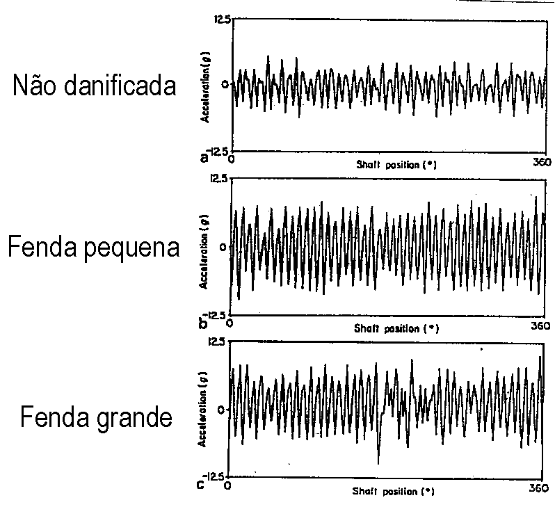
If, in a rotation of a shaft, it travels at an angle of 360º because it does not represent the corresponding vibrations in a circle instead of representing them over time? In this way the defects in shape associated with a given position, they will always appear in the same place making it often easier to identify and making this tool an important diagnostic aid. Next in Figure 13.18, you can see the circular presentation of the waveform in acceleration of the vibrations of a roll with defects in profile.

Vibration analyzer 13 - Figure 13.18 - Vibration analyzer - Circular display of vibrations from a roll of a paper machine with a profile defect
13.7.2. Implementation techniques for circular presentation
There are several possibilities for this approach to the representation of vibrations, namely:
- Simple waveform
- With the synchronous mean of the waveform
- With envelope waveform and peak retention ( PeakVue)
13.7.2.1 - The waveform
This is the simplest form of circular representation and to make it, just have the exact rotation speed of the shaft, what is normally accessible. By itself, it is often difficult to interpret due to interference from other sources of vibration..
13.7.2.2 With the synchronous mean of the waveform
The circular presentation of the vibrations measured with the synchronous mean of the waveform allows, for example, view the profile of each roll of a paper machine, clearly identifying the vibration generator, and causing quality problems on paper.
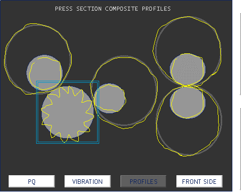 Vibration analyzer 13 - Figure 13.19 - Vibration analyzer - Circular representation of measured vibrations, with the synchronous mean of the waveform in paper machine press rolls, where you can see which roller has the surface that causes vibrations
13.7.2.3 Envelope waveform and peak retention (PeakVue)
The PeakVue waveform can also be displayed in a circular shape as shown in Figure 13.20
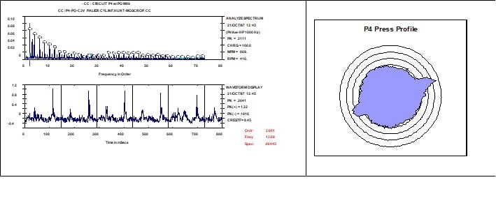 Vibration analyzer 13 - Figure 13.20 - Vibration analyzer - PeakVue Spectrum and Waveform and respective circular representation of a roll of a paper machine press with two shape defects on its surface.
The advantage that this technique has, relative to the synchronous average, is not to need a tachometric sensor. Effectively as PeakVue is a measurement at high frequencies and these are dissipated in the machine's structure, there is no interference phenomenon between the different measurement points. In other words, the vibrations measured at a point are exclusively those at that point.
To see some examples of application of this technique click here.