Vibration analyzer 15 – Spectrum units and scales
Vibration analyzer 15 – Spectrum units and scales
The specific topic dealt with in a vibration analyzer 15, consists of the scale units of the frequency spectrum, a vibration analyzer.
When it takes placeVibration Analysis, in predictive maintenance, to take advantage of the full potential of a vibration analyzer, you need to understand how it works. Therefore, here are presented the concepts of digital signal analysis, currently implemented on an FFT vibration analyzer, from the user's point of view.
We begin by presenting the properties of the Fast Fourier Transform (FFT) on which Vibration Analyzers are based. Then, it shows how these FFT properties can cause some undesirable characteristics in the analysis of the spectrum, like aliasing and breakouts (leakage). Having presented a potential difficulty with the FFT, shows what solutions are used to make vibration analyzers practical tools. Building on this basic knowledge of FFT characteristics makes it simple to get good results with a vibration analyzer on a wide range of vibration problems. measurement.
Here you can see the range ofVibration analyzers made available by D4VIB.
- What is the relationship between time and frequency
- How sampling and scanning works
- What Aliasing is and what effects it has
- How it is used and what the zoom consists of
- How waveform windows are used
- What are averages for
- What is real-time bandwidth
- What overlay processing is for (“overlap”)
- What is order tracking
- What is envelope analysis
- The two-channel functions in the frequency domain
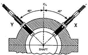
- What Orbit is for
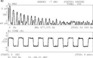
- What are the functions of a channel in the time domain
- What the Cepstro consists of
- What are the units and scales of the spectrum
15 Frequency spectrum units and scales
15.1 Frequency axis and types of vibrations
deterministic signals (signs of a periodic nature, such as the signals measured from a rotating machine, bearings, gear or anything that repeats)
Deterministic stationary signals are composed entirely of sine waves at discrete frequencies. The resolution of frequency analysis is determined by the filter bandwidth used in the analysis., that is, the line width of the FFT analysis. The filter bandwidth should allow the analyzer to distinguish between the two more widely spaced frequency components. This means that there should be only one sinusoid in each filter band at a time.. If that's the case, the power transmitted by the filter is independent of the bandwidth. Therefore, the average frequency spectrum of a deterministic signal must be scaled in terms of root mean square (RMS) or mean square, potency (PWR).
random signals (signals of a random nature that are not necessarily periodic such as cavitation)
Random signals have no obvious periodicity, therefore, frequency analysis cannot determine the "amplitude" at certain frequencies. However, it is possible to measure the r.m.s power level. or power density level in certain frequency bands for these random signals. Random signals have a spectrum that is continuously distributed with frequency.. Consequently, there is a continuous frequency distribution within the spectrum line frequency band. Therefore, the power measured on the line depends on the spectrum resolution, that is, of line width, that is, the parser resolution (B = ∆f × k). For a relatively flat spectrum, it is possible to remove the influence of the filter bandwidth by dividing the transmitted power by the line width. This normalizes the result to a mean square spectral density., commonly called power spectral density (PSD), which is a measure of power per unit of bandwidth.
Transient signals (are not periodic nor randomly stable)
A transient is a signal that starts and ends at zero.. This signal contains a finite amount of energy and, therefore, cannot be characterized in terms of potency, since the potency depends on the duration of the recording: the longer the duration of the measurement, lower average power. Transient signals also have a continuously distributed frequency spectrum.. Consequently, the transmitted power must be normalized in relation to the bandwidth of the line and resized according to the register correctly, regardless of frequency duration. This results in a power unit bandwidth, commonly referred to as energy spectral density (ESD).
| Signal type | spectrum unit | Units |
| Deterministic | RMS (Effective value) PWR(power) | u u2 |
| random | PSD (Power Spectral Density) | u2/Hz |
| Transients | ESD (Spectral Energy Density) | u2s / Hz |
15.2 Vertical axis and logarithmic scales
When you want to see very small vibrations in the presence of very large vibrations, such as, for example, the first symptoms of failures in bearings in an acceleration spectrum, the logarithmic scales are the ones that present the first evidence of what is happening..
Let's look at an example of what could happen. Let's say you have a machine with bearings with some imbalance. The imbalance was diagnosed quite easily.. At the same time, there is a problem in the development of the outer race in the load zone of one of the bearings. as you know, the imbalance creates additional forces on the bearings, especially in the cargo area. Due to the mass of the rotor and the rigidity of the machine, there will be a high amplitude peak in machine operating speed. In the linear graph, a 1X high peak can be seen and practically very little. Due to increased load due to unbalanced condition, rather than a slow evolution over time of wear in a bearing, this bearing will likely go from slightly damaged to complete failure in much less time than usual..
In the linear graph display of the FFT spectra for this machine, maybe you don't even see the appearance of bearing frequencies, as the rollers pass through the defect in the loading zone. These peaks will be very small initially compared to the amplitude of the rotational speed imbalance.
On the analyzer screen / data collector, can be just a pixel, practically part of the noise level. However, if changing from linear to logarithmic presentation, bearing frequencies will be evident, at higher and non-synchronous frequencies.
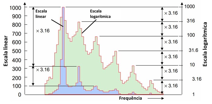
Vibration analyzer 15 – Vibration analyzer – linear scales and logarithmic scales